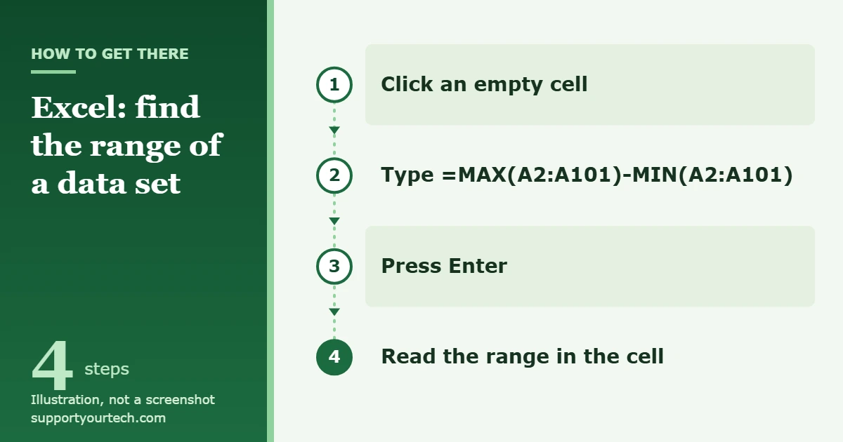
To find the range of a data set in Excel, click an empty cell, type =MAX(A2:A101)-MIN(A2:A101) (using your own cells in place of A2:A101), and press Enter. Excel subtracts the smallest number from the largest and shows the difference, which is the range.
Applies to: Excel for Microsoft 365, Excel 2024, Excel 2021, Excel 2019, and Excel 2016 on Windows and Mac. Checked against Microsoft Support on October 7, 2026.
What the range of a data set means
In statistics, the range is the largest value minus the smallest value. It is the simplest measure of spread: a class with test scores from 62 to 98 has a range of 36, so the top and bottom scores are 36 points apart.
Excel also uses the word “range” for a group of cells, such as A2:A101. That is a different idea. Excel has no function named RANGE, so the statistical range is always built from two functions that every version has: MAX, which returns the largest value in a set, and MIN, which returns the smallest.
Before you start
- Put the values in one column or one row, with one value per cell. The examples below use A2:A101, with a heading in A1.
- Make sure the values are real numbers. MAX and MIN use only the numbers in a reference and ignore empty cells, text, and TRUE/FALSE values.
- Look for stray entries such as a total at the bottom of the column. The range depends on just two cells, so one wrong value changes the answer.
Find the range with one formula
- Click an empty cell outside your data, for example C2. This is where the answer will appear.
- Type =MAX(A2:A101)-MIN(A2:A101). Change A2:A101 to the cells that hold your numbers. You can also type =MAX(, drag across the cells with the mouse, type ), and repeat for the MIN part.
- Press Enter. The cell shows a single number: the distance between the highest and lowest values.
- Type a label such as Range in the cell to the left so anyone reading the sheet knows what the number is.
If your numbers sit in two separate blocks, list both inside each function: =MAX(A2:A101,C2:C101)-MIN(A2:A101,C2:C101). Each function accepts up to 255 arguments.
Show the minimum and maximum in separate cells
Splitting the calculation makes it easier to check, because you can see which two values produce the range.
- In C2, type =MAX(A2:A101) and press Enter. The cell shows the largest value.
- In C3, type =MIN(A2:A101) and press Enter. The cell shows the smallest value.
- In C4, type =C2-C3 and press Enter. The result matches the one-formula method.
Check the range without a formula
In Excel for Microsoft 365, Excel 2024, and Excel 2021 on Windows, the status bar at the bottom of the window can show the two endpoints for any cells you select.
- Right-click the status bar.
- Select Minimum and Maximum. Neither is turned on by default; Average, Count, and Sum are.
- Select your data cells. The status bar now shows the minimum and maximum, and you can subtract one from the other in your head.
In Excel for the web, select the arrow next to the last status bar entry and choose Minimum and Maximum there. This is a quick check only; nothing is saved in the sheet.
Find the range for one group or without extreme values
The MAXIFS and MINIFS functions return the largest or smallest value among the cells that meet a condition. Microsoft lists them for Excel 2019 and later and for Microsoft 365; Excel 2016 does not have them.
One group. With region names in A2:A101 and sales in B2:B101, this returns the range for the East region only:
=MAXIFS(B2:B101,A2:A101,”East”)-MINIFS(B2:B101,A2:A101,”East”)
Leaving out extreme values. If you know that values of 900 or more and values of 5 or less are data-entry mistakes, compare the column against itself:
=MAXIFS(A2:A101,A2:A101,”<900″)-MINIFS(A2:A101,A2:A101,”>5″)
The first range in each function is where Excel looks for the answer, the second is the range it tests, and the text in quotation marks is the test. All the ranges inside one function must be the same size and shape, or Excel returns a #VALUE! error.
Excel 2016. Use MAX and MIN with IF instead: =MAX(IF(A2:A101=”East”,B2:B101))-MIN(IF(A2:A101=”East”,B2:B101)). This is an array formula, so in Excel 2016 confirm it with Ctrl+Shift+Enter rather than Enter alone. Current versions accept it with Enter.
Find the range of filtered or visible rows only
MAX and MIN include rows that a filter has hidden. To measure only what is showing, use SUBTOTAL:
=SUBTOTAL(104,A2:A101)-SUBTOTAL(105,A2:A101)
Function number 104 means MAX and 105 means MIN. SUBTOTAL always leaves out rows removed by a filter, and the 100-series numbers also leave out rows you hid by hand. If you want hand-hidden rows counted, use 4 and 5 instead.
Find the range when the data contains error values
If any cell in the reference holds an error such as #N/A, MAX and MIN return an error too. AGGREGATE can skip those cells:
=AGGREGATE(4,6,A2:A101)-AGGREGATE(5,6,A2:A101)
The first argument picks the calculation (4 is MAX, 5 is MIN) and the second, 6, tells Excel to ignore error values. Use 7 instead of 6 to ignore hidden rows as well. Microsoft notes that AGGREGATE is designed for columns of data, not for data laid out across a row.
Keep the range correct as you add rows
A formula that points at A2:A101 will not notice a value typed in A102. An Excel table fixes that.
- Select any cell in your data and press Ctrl+T.
- Confirm that My table has headers is checked and select OK. Excel names the first table in a workbook Table1.
- Write the formula with the table and column name, for example =MAX(Table1[Sales])-MIN(Table1[Sales]) when the column heading is Sales.
References written this way adjust on their own whenever rows are added to or removed from the table.
Use LARGE and SMALL to drop the top and bottom values
=LARGE(A2:A101,1)-SMALL(A2:A101,1) gives the same answer as MAX minus MIN, because LARGE with 1 returns the largest value and SMALL with 1 returns the smallest. The advantage is the second argument: change both 1s to 2 and Excel measures from the second-largest to the second-smallest value, which is a fast way to see how much a single extreme value at each end is stretching the range.
How to confirm the result
- Compare the answer with the separate MAX and MIN cells, or with the Minimum and Maximum figures on the status bar.
- Sort the column and look at the first and last values. They should be the two numbers the formula used.
- Test with a small set you can check by eye. For 12, 7, 31, 18, and 25, the maximum is 31, the minimum is 7, and the range is 24.
To undo the calculation, delete the formula cell. Formulas never change the data they read.
Troubleshooting
The result is 0
MAX and MIN both return 0 when the reference contains no numbers, so 0 minus 0 gives 0. This usually means the values are numbers stored as text, which Excel marks with a small green triangle in the corner of the cell. Select the cells, select the warning button that appears, and choose Convert to Number. A range of 0 is also correct when every value is identical.
The result looks too small
If only some cells are stored as text, MAX and MIN silently skip them and work from the rest. Convert those cells the same way, then check the formula again.
The formula returns an error value
An error inside the data passes through MAX and MIN. Fix the source cell, or switch to the AGGREGATE formula above. A #VALUE! error from MAXIFS or MINIFS means the ranges inside the function are different sizes.
Excel does not recognize MAXIFS or MINIFS
These functions need Excel 2019 or later, or Microsoft 365. In Excel 2016, use the MAX and IF version.
The range does not change when the data changes
The workbook is probably set to manual calculation. Go to File > Options > Formulas and, under Workbook Calculation, select Automatic. To recalculate once without changing the setting, press F9.
The range is far larger than expected
Look at the MAX and MIN results on their own. A subtotal row caught in the reference, a value typed with an extra digit, or mixed units (dollars in some rows, thousands of dollars in others) are the usual causes.
When the range is not the right measure
Because it uses only two values, the range says nothing about how the rest of the data is distributed, and one outlier can dominate it. The interquartile range measures the middle half of the data instead: =QUARTILE.INC(A2:A101,3)-QUARTILE.INC(A2:A101,1) subtracts the first quartile (25th percentile) from the third (75th percentile). Our guide on how to find the interquartile range in Excel covers it step by step, and finding the standard deviation of a data set shows a measure that uses every value.
Frequently asked questions
Is there a RANGE function in Excel?
No. Microsoft’s alphabetical function list has no function called RANGE. Subtract MIN from MAX instead.
Do blank cells or text affect the range?
Not directly. Within a reference, MAX and MIN ignore empty cells, text, and logical values. A blank is not treated as zero, so it will not pull the minimum down.
Does the formula work with negative numbers?
Yes. The range is still the maximum minus the minimum. For values from -8 to 15, the range is 15 minus -8, which is 23.
Can I find the range of data in a row instead of a column?
Yes. MAX and MIN accept any reference, so =MAX(B2:M2)-MIN(B2:M2) works. Only the AGGREGATE version is meant for columns.
Which Excel versions have MAX and MIN?
Microsoft’s reference pages list both for Excel 2016 through Excel 2024 and Microsoft 365, on Windows and Mac. Only the conditional MAXIFS and MINIFS functions need Excel 2019 or later.
Once the range is in place, add the MAX and MIN cells beside it so readers can see the endpoints. Microsoft documents the two functions on its MAX function and MIN function pages.
Related: how to calculate a 95% confidence interval in Excel.
Related: How to Rank in Excel Highest to Lowest.
Related: how to create a range in Excel.

Matt Jacobs has been working as an IT consultant for small businesses since receiving his Master’s degree in 2003. While he still does some consulting work, his primary focus now is on creating technology support content for SupportYourTech.com.
His work can be found on many websites and focuses on topics such as Microsoft Office, Apple devices, Android devices, Photoshop, and more.