How to Pull a Random Sample in Excel

To pull a random sample in Excel, type =RAND() in an empty helper column next to your data, fill it down every row, convert the results to fixed numbers with Paste Options > Values Only, and then sort the list with Data > Sort Smallest to Largest. The first rows of the shuffled list are your sample: keep the top 10 for a sample of 10, the top 50 for a sample of 50, and so on.

Applies to: Excel for Microsoft 365, Excel 2024, Excel 2021, Excel 2019 and Excel 2016 (helper-column method); the one-formula method needs Excel for Microsoft 365, Excel 2024 or Excel 2021. Checked against Microsoft Support on October 7, 2026.

Before you start

A random sample is a smaller set of rows chosen by chance, so that every row has the same opportunity to be picked. People use one to choose survey recipients, to pick records for an audit or a quality check, or to test a calculation on part of a long list. A few minutes of preparation prevents most problems:

• Work on a copy. The main method reorders your rows. Microsoft recommends making a copy of the workbook before you replace formulas with their results, and a copy also protects the original row order.
• Keep the headings in one row. Microsoft’s sorting guidance says column headings should sit in a single row. Split headings across two rows can end up sorted into the data.
• Unhide hidden rows and columns. Hidden rows and columns are not moved when you sort, so unhide them first or part of each record can be left behind.
• Keep the list in one block. Every record should be one row, with no completely blank rows or columns splitting the list, so Excel treats it as a single range.
• Decide the sample size. Know how many rows you want before you begin. For a percentage, multiply the number of data rows by the percentage: 10% of 500 rows is 50 rows.
• Add an ID column if the original order matters. If the list has no column you could sort by later to restore the starting order, add a column numbered 1, 2, 3 and so on before you shuffle.

Pull a random sample with a RAND helper column

This method works in every current version of Excel and keeps each record intact, because whole rows move together. A helper column is simply an extra column that you add to do a job and delete afterward. The example assumes headings in row 1 and data in columns A to C, with column D empty.

1. Label the helper column. Click the first empty cell to the right of your headings (D1 in the example) and type Random. The helper column now has a heading like the other columns.
2. Enter the formula. In the first data row of that column (D2), type =RAND() and press Enter. The function takes no arguments. Excel shows a decimal number that is greater than or equal to 0 and less than 1.
3. Fill the formula down to the last record. Select D2, then drag the fill handle (the small square at the bottom-right corner of the selected cell) down to the last row of data. You can also select D2 through the last row and press Ctrl+D, or select Home > Fill > Down. Every row should now show a different decimal.
4. Freeze the random numbers. Select the filled cells in the helper column and select Copy. With the same cells still selected, select Paste, select the arrow next to Paste Options, and then select Values Only. The cells now hold plain numbers instead of formulas, so they stop changing. To check, click one of them: the formula bar shows a number, not =RAND().
5. Sort by the helper column. Click any single cell in the Random column. On the Data tab, in the Sort & Filter group, select Sort Smallest to Largest. Excel reorders the whole list by the random numbers, which shuffles your records. (Sort Largest to Smallest gives an equally random order.)
6. Take the first rows as the sample. Select as many rows from the top of the shuffled list as your sample size, copy them, and paste them on a new worksheet. Add the header row above them if you need the labels.
7. Clean up. Delete the Random column from the copy you are keeping, or leave it in place as a record of how the sample was drawn.

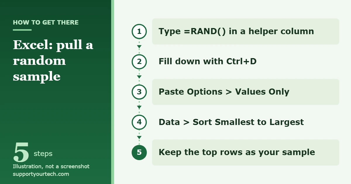
Because every record appears exactly once in the shuffled list, this method cannot pick the same row twice. Statisticians call that sampling without replacement, and it is what most surveys and audits need.

If you want more control over the sort, select Data > Sort instead. In the dialog box, make sure My data has headers is checked, choose your Random column in the Sort by box, leave Sort On set to Cell Values, set Order to Smallest to Largest, and select OK.

Why you should freeze the numbers first

Microsoft’s documentation for the RAND function states that a new random number is returned every time the worksheet is calculated. Calculation happens when you enter data in another cell, when you press F9, and after other changes to the sheet. Microsoft’s sorting article adds that when sorted data contains formulas, the formula results may change when the worksheet recalculates.

In practice, this means that a live =RAND() column gives you a different shuffle every time something changes, and you cannot reproduce or document the sample you drew. Converting the column to values before sorting fixes the order permanently. You can still take a fresh sample later: put =RAND() back in the column, fill it down, freeze it, and sort again.

If you only need to freeze a single cell, Microsoft documents a keyboard route: press F2 to edit the cell, press F9, and then press Enter. For a whole column, the copy and Values Only route in step 4 is faster. If you would like more background on RAND and its whole-number relative, see our guide on how to randomly generate numbers in Excel.

Pull a random sample with one formula (Microsoft 365, Excel 2024 and Excel 2021)

Newer versions of Excel can build the sample in a separate place and leave the original list untouched. Microsoft lists RANDARRAY and SORTBY as available in Excel for Microsoft 365, Excel 2024 and Excel 2021. TAKE is listed for Excel for Microsoft 365 and Excel 2024 only, so Excel 2021 users should use the second formula below.

Microsoft 365 and Excel 2024: shuffle and keep the top rows

1. Pick an empty area. Click a cell with enough empty cells below it and to its right to hold the sample, for example F2 or a cell on a new worksheet.
2. Type the formula. For data in A2:C101 and a sample of 10 rows, enter =TAKE(SORTBY(A2:C101,RANDARRAY(ROWS(A2:C101))),10) and press Enter.
3. Check the result. Ten complete records appear, starting in the cell where you typed the formula. Excel fills the neighboring cells automatically, which Microsoft calls spilling.
4. Freeze the sample. Select the results and select Copy. Select Paste, then the arrow next to Paste Options, then Values Only. Until you do this, the sample is redrawn each time the worksheet calculates.

Here is what each part does. RANDARRAY returns a column of random decimals, and ROWS tells it how many to make by counting the rows in your data. SORTBY sorts your range by those random numbers, which shuffles it. TAKE then returns the number of rows you ask for from the start of the shuffled result. Change the range to match your data and change 10 to your sample size. Leave the header row out of the range.

Excel 2021: shuffle the whole list

In an empty area, enter =SORTBY(A2:C101,RANDARRAY(ROWS(A2:C101))). Excel returns the entire list in random order. Copy the results, paste them with Values Only, and keep the first rows you need. This formula also works in Microsoft 365 and Excel 2024.

The Sampling tool in the Analysis ToolPak

Excel also includes a Sampling tool as part of the Analysis ToolPak, an add-in that has to be loaded before its tools appear. Microsoft describes the tool as creating a sample from a population by treating the range you give it as the population. It can also sample periodically, for example taking every fourth value from quarterly figures.

To load the add-in in Excel for Windows:

1. Select the File tab, select Options, and then select the Add-Ins category.
2. In the Manage box, select Excel Add-ins, and then select Go.
3. In the Add-Ins box, check the Analysis ToolPak check box, and then select OK.

On a Mac, Microsoft’s instructions are to go to Tools > Excel Add-ins, check Analysis ToolPak, and select OK. Once the add-in is loaded, select Data Analysis on the Data tab and choose the Sampling tool from the list. Microsoft’s page on how to load the Analysis ToolPak in Excel covers both platforms.

Microsoft describes the tool as placing values from the input range into an output range, so it is a better fit for sampling a column of values than for pulling complete multi-column records. Microsoft’s description also does not promise that each value is picked only once. If you need whole rows, or need to be sure that no row is chosen twice, use the helper-column or SORTBY method instead. Microsoft also notes that the data analysis tools work on only one worksheet at a time. Our walkthrough on how to use data analysis in Excel introduces the other tools in the add-in.

Which method should you use?

Method	Excel versions	Best for	Keep in mind
RAND helper column and sort	Microsoft 365, 2024, 2021, 2019, 2016	Any list, any version; keeps whole records together	Reorders the list, so work on a copy
TAKE with SORTBY and RANDARRAY	Microsoft 365, 2024	Leaving the source list untouched	Redraws on every calculation until pasted as values
SORTBY with RANDARRAY	Microsoft 365, 2024, 2021	Shuffling a full list in a new location	Returns every row; you keep the first ones
Analysis ToolPak Sampling tool	Versions with the add-in loaded	Sampling values from one column, or every nth value	Add-in must be loaded first

Sample evenly from groups

A plain random sample can, by chance, include too many rows from one region, department or month and too few from another. If each group must be represented, you can draw a fixed number of rows from every group. This is called stratified sampling.

1. Add the Random column and freeze it as values, as in steps 1 to 4 of the main method.
2. Select Data > Sort. In the Sort by box, choose the column that holds the group, such as Region.
3. Select Add Level, and in the new row choose the Random column with Order set to Smallest to Largest. Select OK.
4. The rows are now grouped, and shuffled inside each group. Take the first rows of each group, for example the first five from every region.

Confirm it worked, or undo it

• Check that records stayed together. Find one record you know and confirm that every cell in its row still belongs to it, for example that a customer’s name is still beside the correct order number.
• Check the count. Compare the first and last row numbers of the rows you copied to confirm the sample holds the number of records you intended.
• Check that the order is fixed. Press F9. If the numbers in the Random column change, they are still formulas and need to be pasted as values.
• Undo the sort. Select Undo right after sorting to return the rows to their previous order. If you have already saved and closed the workbook, sort by your ID column, or go back to the copy you made.
• Restore a formula. If you pasted values over a formula by mistake, Microsoft’s advice is to select Undo immediately after pasting.

Troubleshooting

Excel asks whether to expand the selection

If you selected the whole Random column, or several cells in it, instead of a single cell, Excel asks whether to include the neighboring columns. Choose Expand the selection so entire rows move together. Continue with the current selection would sort only the helper column and leave your records in their original order, so the result would not be a shuffled list. Microsoft’s guide to sorting data in a range or table explains the choice.

The random numbers keep changing

That is how RAND is designed to behave. Paste the helper column as values (step 4) to stop it. Switching the workbook to manual calculation is not a reliable fix, because the numbers still change the next time the sheet is calculated.

The numbers do not change at all, or every row shows the same number

The workbook is probably set to manual calculation. Select File > Options, select Formulas, and under Workbook Calculation choose Automatic. To calculate once without changing the setting, press F9, or select Calculate Now in the Calculation group on the Formulas tab.

The fill handle is missing

Select File > Options, select Advanced, and under Editing Options check the Enable fill handle and cell drag-and-drop box. You can also skip the handle and use Ctrl+D or Home > Fill > Down.

The header row was sorted into the data

Select Undo, then sort with Data > Sort and make sure My data has headers is checked before you select OK.

The one-formula method returns an error

Check three things. First, the cells below and to the right of the formula must be empty, because the results need room to spill. Second, an error can mean that your version of Excel does not have one of the functions: TAKE needs Microsoft 365 or Excel 2024, and SORTBY and RANDARRAY need Excel 2021 or later. Third, the two ranges inside the formula must match, because Microsoft requires all SORTBY arguments to be the same size. If your data is in A2:C101, ROWS must also refer to A2:C101.

Data Analysis is not on the Data tab

The Analysis ToolPak is not loaded. Follow the three steps in the Sampling tool section. If Analysis ToolPak is not listed in the Add-Ins box, Microsoft says to select Browse to locate it, and to select Yes if Excel reports that the add-in is not currently installed. On a work or school computer where add-ins are managed for you, you may need to ask your IT administrator.

Some rows did not move

Hidden rows are not moved by a sort, and a completely blank row or column can make Excel treat the list as two separate ranges. Select Undo, unhide everything, remove the blank row or column, and sort again.

Frequently asked questions

Can the same row appear twice in my sample?

Not with the helper-column method or the SORTBY formulas. Both shuffle the list and take rows from the top, and each record appears once in the shuffled list. Duplicates in the sample are possible only if the same record was already entered more than once in your source data.

How do I pull a different sample next time?

With the helper column, enter =RAND() again, fill it down, paste it as values and sort. With the one-formula method, press F9 to redraw the sample, then paste the new result as values.

How do I take a 10% sample?

Work out the number of rows first. Multiply the number of data rows by 0.1 and round to a whole number, then keep that many rows from the top of the shuffled list or use the number as the last argument in TAKE. For 2,000 rows, a 10% sample is 200 rows.

Does this work if my data is formatted as an Excel table?

Yes for the helper column: add the Random column to the table, freeze it, and sort by it. For the one-formula method, type the formula in a cell outside the table. Microsoft notes that SORTBY and RANDARRAY accept table references, and that the results resize automatically as table rows are added or removed.

Is a random sample always representative?

No. Random selection removes your own bias from the choice, but a small sample can still differ from the full list by chance. Larger samples vary less. When specific groups must be included, use the grouped method above.

Can I draw the sample from data in another workbook?

The helper-column method works wherever the data lives, so copying the list into the current workbook first is the simplest route. Microsoft notes that formulas such as SORTBY and RANDARRAY have limited support between workbooks, and work only while both workbooks are open.

Once your sample is on its own worksheet, save the workbook under a new name so the drawn sample and the full list are both preserved, and note the date and sample size alongside it if you may need to show later how it was selected.