How to Calculate Commission in Excel

To calculate a sales commission in Excel, multiply the sales amount by the commission rate. With sales in B2 and the rate in C2, type =B2*C2 in D2 and press Enter, then drag the fill handle down to copy the formula to the other rows. Plans with a quota, a threshold or tiers need one extra function, covered below.

Applies to: Microsoft Excel for Windows and Mac (Microsoft 365 and other current desktop versions; XLOOKUP is not available in Excel 2016 or Excel 2019). Checked against Microsoft Support on October 7, 2026.

Before you start

A commission formula is only as good as the rule behind it, so read the compensation plan first and answer three questions:

• What is the commission paid on? Total sales, sales above a quota, or profit (sales minus cost).
• Is there one rate or several? One flat rate, a different rate for each person or product, or tiers that change as sales grow.
• If there are tiers, how do they apply? In a whole-amount plan, reaching a tier changes the rate on every dollar. In a marginal plan, each slice of sales is paid at its own rate, the way income tax brackets work. The two give very different results.

Set up the sheet with one row per salesperson or per sale and a header in row 1. The examples in this article use Rep in column A, Sales in column B, Rate in column C and Commission in column D.

How to calculate a basic commission in Excel

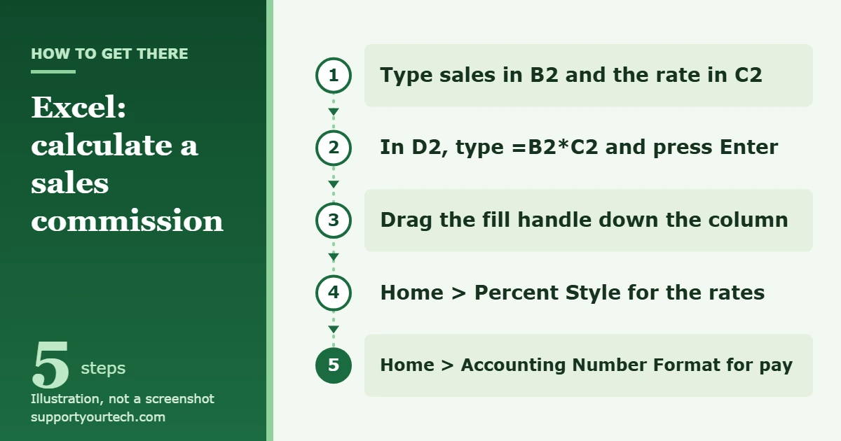
1. Enter the sales amount. Click cell B2 and type the sales figure as a plain number, such as 12000.
2. Enter the commission rate. Click C2 and type the rate with a percent sign, such as 5%. Excel stores this as 0.05 and shows it as a percentage.
3. Type the formula. Click D2, type =B2*C2 and press Enter (Return on a Mac). The asterisk is Excel’s multiplication sign. D2 shows 600.
4. Copy the formula down. Select D2 and drag the fill handle, the small square at the lower-right corner of the cell, down to the last row of data. You can also select D2 together with the cells below it and press Ctrl+D, or choose Home > Fill > Down. Each row now multiplies its own sales by its own rate.
5. Format the results. Select the commission cells and, on the Home tab in the Number group, click Accounting Number Format. For the rate column, click Percent Style in the same group.

Use one commission rate for every row

If everyone earns the same rate, keep it in a single cell, for example F1, so that it only has to be changed in one place. In D2 type =B2*$F$1 and fill the formula down.

The dollar signs make F1 an absolute reference. Cell references are relative by default, which means they shift when a formula is copied: without the dollar signs, row 3 would look for a rate in F2, find an empty cell and return 0. To add the dollar signs quickly on Windows, select the reference in the formula bar and press F4, which switches between the reference types. You can also simply type them.

Pay commission only after a quota or threshold

Two common rules sound alike but pay differently. The examples assume a 10,000 quota and the rate in F1.

• Commission on everything once the quota is met: =IF(B2>=10000,B2*$F$1,0). IF checks a condition and returns one value when it is true and another when it is false. At 5%, sales of 12,000 pay 600 and sales of 9,999 pay 0.
• Commission only on the amount above the threshold: =MAX(0,B2-10000)*$F$1. MAX returns the larger of its arguments, so a negative difference becomes 0. At 5%, sales of 12,000 pay 100 and sales of 8,000 pay 0.

Putting the quota in its own cell, such as F2, and writing $F$2 in place of 10000 makes next year’s change a one-cell edit.

Calculate tiered commission with a rate table

For tiers, build a small table on the same sheet. The first column holds the sales amount where each tier starts, and it must begin at 0 and be sorted from smallest to largest. The examples use this table in H2:I4.

Sales from (column H)	Rate (column I)
0	3%
10,000	5%
25,000	7%

Whole-amount tiers with VLOOKUP

When the tier reached sets the rate for all sales, use =B2*VLOOKUP(B2,$H$2:$I$4,2,TRUE). VLOOKUP searches the first column of the table for the sales figure and returns the rate from column 2. TRUE asks for an approximate match, which picks the tier whose starting amount is at or just below the sales figure. Sales of 12,000 pay 5%, or 600. Sales of 30,000 pay 7%, or 2,100. Sales of exactly 10,000 land in the 5% tier.

Microsoft’s VLOOKUP function reference notes that an approximate match assumes the first column is sorted, and that the function returns #N/A when the lookup value is smaller than the smallest value in that column. That is why the table starts at 0.

The same lookup with XLOOKUP

In versions of Excel that include XLOOKUP, you can write =B2*XLOOKUP(B2,$H$2:$H$4,$I$2:$I$4,,-1). The final -1 is the match mode that returns the next smaller item when there is no exact match. Leave the fourth argument empty, as shown, or put a message there to display when nothing is found. XLOOKUP is not available in Excel 2016 or Excel 2019, so use VLOOKUP if the workbook will be opened in those versions.

Marginal tiers, where each slice has its own rate

For a marginal plan, add the commission earned in each tier:

=MIN(B2,10000)*3%+MAX(0,MIN(B2,25000)-10000)*5%+MAX(0,B2-25000)*7%

MIN caps each slice at the top of its tier and MAX stops a slice from going below zero. For sales of 30,000 the result is 300 + 750 + 350 = 1,400, compared with 2,100 under the whole-amount rule. For sales of 12,000 it is 300 + 100 = 400.

A shorter formula works if you add a third column to the table (J2:J4) containing how much the rate rises at each tier: 3%, 2% and 2% here. Then use =SUMPRODUCT((B2>$H$2:$H$4)*(B2-$H$2:$H$4)*$J$2:$J$4). It returns the same 1,400 for sales of 30,000, and adding a tier only means adding a table row and widening the three ranges, which must stay the same size.

Other common commission setups

• A different rate for each person or product. List the names in L2:L4 and their rates in M2:M4, then use =B2*VLOOKUP(A2,$L$2:$M$4,2,FALSE). FALSE asks for an exact match, so a misspelled name returns #N/A instead of someone else’s rate.
• Commission on profit. Put the cost in its own column and subtract it first. With sales in B2, cost in C2 and the rate in F1, use =(B2-C2)*$F$1. The parentheses matter, because Excel multiplies before it subtracts.
• Total commission per person. When the sheet lists individual sales, =SUMIF(A2:A50,”Ana”,D2:D50) adds the commission amounts in column D for every row where column A says Ana.
• Rounding to cents. Number formats change only what is displayed. To store a rounded amount, wrap the formula in ROUND, for example =ROUND(B2*C2,2).

Which formula fits your plan?

Plan rule	Formula for D2
Rate stored on each row	=B2*C2
One rate for everyone, in F1	=B2*$F$1
All sales, but only once quota is met	=IF(B2>=10000,B2*$F$1,0)
Only sales above a threshold	=MAX(0,B2-10000)*$F$1
Tier reached sets the rate for all sales	=B2*VLOOKUP(B2,$H$2:$I$4,2,TRUE)
Each slice of sales has its own rate	The MIN and MAX formula, or SUMPRODUCT

Format the rates and commission amounts

For rates, select the cells and click Percent Style in the Number group on the Home tab, or press Ctrl+Shift+%. To show a rate such as 2.5%, press Ctrl+1 to open Format Cells, choose Percentage in the Category list and set Decimal places to 1 or 2.

For money, click Accounting Number Format or press Ctrl+Shift+$ for the Currency format. Accounting lines up the currency symbols and decimal points in a column and shows zeros as dashes, while Currency keeps the symbol next to the first digit.

Check that the commission is right

1. Work out two or three rows on a calculator and compare them with the sheet.
2. Test the edges. Type a sales figure just below, exactly on and just above each quota or tier boundary and confirm that each result matches the written plan.
3. For a long formula, select its cell and go to Formulas > Formula Auditing > Evaluate Formula, then click Evaluate repeatedly to watch Excel calculate one part at a time.

A formula never overwrites the sales data it reads, so a mistake is easy to undo: correct the formula in D2 and fill it down again.

Troubleshooting commission formulas

• The commission is 100 times too large. The rate is probably the number 5, not 5%. Applying the Percentage format to a cell that already contains 5 turns it into 500%, because Excel multiplies existing numbers by 100. Retype the rate as 5% or as 0.05.
• Row 2 is right but the rows below show 0 or wrong amounts. A reference to a single rate cell or to the tier table is missing its dollar signs. Fix the formula in D2 and fill it down again.
• #N/A. With a tier table, the sales figure is lower than the first value in the table, or a sales cell holds a negative number. With an exact-match lookup, the name is not in the table or is spelled differently.
• The wrong tier is returned. The first column of the tier table is not sorted from smallest to largest, or its amounts are stored as text.
• #NAME?. A function name is misspelled, or the workbook uses XLOOKUP in a version of Excel that does not have it.
• #VALUE! from SUMPRODUCT. The ranges in the formula are not all the same size.
• Sales figures are ignored or show a green triangle. The numbers are stored as text, which is common in data exported from another system. Select the cells, open the alert that appears beside them and choose Convert to Number.
• ##### appears in place of a result. The column is too narrow for the formatted number. Double-click the right edge of the column heading to widen it.
• There is no fill handle to drag. Go to File > Options > Advanced and select Enable fill handle and cell drag-and-drop.
• Results do not update when sales change. Go to File > Options > Formulas and, under Workbook Calculation, choose Automatic.
• You cannot edit the formula cells. A workbook supplied by your employer may be protected so that only certain cells can be changed. Ask the person who owns the file to update the formula or to give you an editable copy.

Frequently asked questions

What is the formula for commission in Excel?

Sales multiplied by the rate. With sales in B2 and a percentage rate in C2, the formula is =B2*C2. To use a fixed rate without a rate cell, type it into the formula, as in =B2*5%.

Do I need to divide the rate by 100?

Not when the rate is entered as a percentage. Excel stores 5% as 0.05, so =B2*C2 is already correct. Divide by 100 only if the rate cell holds a plain number such as 5. Our guide on how to multiply by a percentage in Excel explains the difference.

How do I add a base salary or a bonus to the commission?

Add it to the end of the formula. With base pay in E2, =E2+B2*C2 returns total pay. For a fixed 500 bonus when sales reach 20,000, use =B2*C2+IF(B2>=20000,500,0).

How do I subtract a draw or an advance?

Put the amount already paid in its own column and subtract it from the commission, for example =D2-E2. Keeping the draw in a separate cell leaves a record of how the net figure was reached.

Should I use nested IF functions for tiers?

Excel lets you nest IF functions, and for two tiers that is readable. Beyond that, a rate table with VLOOKUP or XLOOKUP is easier to check and to update, because a rate change is made in the table without rewriting every formula.

Can I use these formulas in Excel for the web or on a Mac?

The formulas are the same wherever a function is available. The keyboard shortcuts and the File > Options paths in this article are the ones Microsoft documents for the Windows desktop app, so menus may differ elsewhere.

Once the formulas match your plan, save a copy of the workbook as a template for the next pay period and paste in new sales figures each time. Review the IF, VLOOKUP and tier ranges whenever the plan’s quota or rates change.