How to Use Absolute Cell Reference in Excel

To use an absolute cell reference in Excel, type a dollar sign before both the column letter and the row number, like $E$1, then copy or fill the formula. Every copy keeps pointing at E1 while the other references move. The fastest way to add the dollar signs is to click the reference in the formula bar and press F4 on Windows or Command + T on a Mac.

Applies to: Excel for Microsoft 365 (Windows and Mac), Excel 2024, Excel 2021, Excel 2019, Excel 2016 and Excel for the web. Dollar-sign references work the same way in all of them; only the shortcut key differs. Microsoft’s own summary is on its page about switching between relative, absolute and mixed references.

What the dollar sign does

Excel stores a normal reference like E1 as a position: “four columns to the right and one row up from here,” for example. When you copy the formula, that position moves with it. This is called a relative reference, and it’s the default.

A dollar sign freezes the part of the address that follows it. Put one before the column letter, the row number, or both. Here’s how each form changes when you copy a formula two rows down and two columns to the right: That $ only locks the address; to show a $ in front of money amounts instead, see adding dollar signs to numbers in Excel.

You type	Type	After copying 2 down, 2 right	What stays fixed
A1	Relative	C3	Nothing
$A$1	Absolute	$A$1	Column and row
A$1	Mixed	C$1	Row only
$A1	Mixed	$A3	Column only

Use an absolute reference when every copy of a formula needs the same single value: a tax rate, a commission rate, an exchange rate or a grand total. The dollar sign has nothing to do with money. It shows up only in the formula, never in the result. A year-by-year savings table is a good practice case, because every row has to point at the same rate and starting balance when you build a compound interest table in Excel.

Use an absolute reference, step by step

This example works out a 5% commission for a small sales team. If you want to follow along, type these into a blank sheet:

• A1: Name, B1: Sales, C1: Commission
• A2 to A4: Alex, Jordan, Priya
• B2 to B4: 4200, 3150, 5800
• D1: Rate, and E1: 5%

1. Select the first result cell. Click C2, next to Alex’s sales.
2. Start the formula. Type =B2*E1, but don’t press Enter yet.
3. Lock the rate. With the cursor still touching E1 in the formula, press F4 (Windows) or Command + T (Mac). The formula changes to =B2*$E$1. You can also type the two dollar signs yourself.

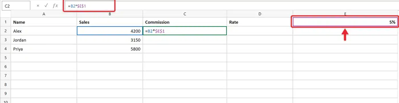
4. Press Enter. C2 shows 210.
5. Copy the formula down. Click C2, then drag the small square at its bottom-right corner (the fill handle) down to C4. Double-clicking that square also works when the column next to it has data. If the fill handle is new to you, see how to use the fill handle in Excel.
6. Check a copied cell. Click C4. The formula bar should read =B4*$E$1: the sales reference moved to row 4, but the rate stayed on E1. The result is 290.

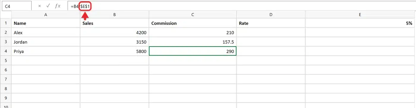
Without the dollar signs, C3 would read =B3*E2 and C4 =B4*E3. Those cells are empty, so the commissions would show 0. That row of zeros (or a #VALUE! error if the moved reference lands on text) is the classic sign of a missing absolute reference.

The payoff comes later: change E1 to 6% and every commission updates at once.

Three ways to add the dollar signs

F4 on Windows

Click in the formula bar (or double-click the cell, or press F2), put the cursor on or right after the reference, and press F4. Each press moves to the next form:

1. First press: $E$1 (absolute)
2. Second press: E$1 (row locked)
3. Third press: $E1 (column locked)
4. Fourth press: E1 (back to relative)

To change several references at once, select that part of the formula text first, then press F4. On many laptops the top row of keys controls volume or brightness by default, so hold Fn and press F4.

Command + T on a Mac

Select the reference in the formula bar and press Command + T. It cycles through the same four forms in the same order. More Mac detail, including what to do when the shortcut doesn’t respond, is in how to make an absolute reference in Excel on Mac.

Type the dollar signs

Typing $ (Shift + 4 on a US keyboard) works in every version, including Excel for the web, Excel on a phone or tablet, and keyboards without function keys. In Excel for the web, try F4 first; if nothing changes, typing is the reliable fallback.

Which to choose: use the shortcut while you’re building a formula, and type the dollar signs when you’re fixing one reference inside a long formula or when the shortcut isn’t available.

Lock a whole range

Ranges need dollar signs on both ends. Select the whole range in the formula and press F4 once to change both halves together.

• Lookup tables: In =VLOOKUP(A2,$H$2:$I$50,2,FALSE), the table stays put while A2 moves down row by row. Forgetting this is why lookups work in the first row and fail lower down. The full method is in how to do a VLOOKUP in Excel.
• Percentage of a total: With values in B2:B9 and the total in B10, type =B2/$B$10 in C2 and fill down.
• Running total: =SUM($B$2:B2) anchors the start of the range and lets the end grow as you fill down.

When to use a mixed reference instead

A mixed reference is the right tool when one formula fills a grid both down and across. Picture a price list in column A (A3:A6) and exchange rates for three currencies across row 2 (B2:D2). In B3, type =$A3*B$2 and fill it across to D3, then down to row 6.

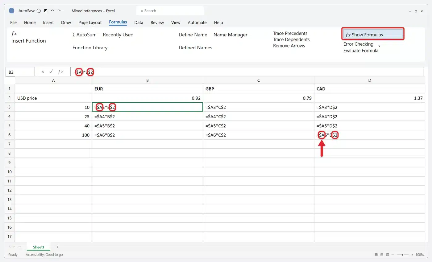
• $A3 keeps every formula reading prices from column A, while the row changes.
• B$2 keeps every formula reading rates from row 2, while the column changes.

If you used $A$3 and $B$2 here, every cell would show the same number. A multiplication table built with =$A2*B$1 works the same way.

A readable alternative: name the cell

A name behaves like an absolute reference and is easier to read. Click E1, click the Name Box (the box showing “E1” to the left of the formula bar), type Rate and press Enter. Now =B2*Rate works in any cell and never shifts. Names can’t contain spaces, so use something like TaxRate or Tax_Rate. To edit or delete names later, go to Formulas > Name Manager. See Microsoft’s guide to defining and using names in formulas.

Other sheets and Excel tables

Another sheet: Put the sheet name in front, for example =B2*Settings!$B$1. Typing =B2*, clicking the other sheet’s tab, clicking the cell and pressing F4 builds it for you. Sheet names with spaces need quotes, as in ='Rate Table'!$B$1. Linking to other workbooks is covered in referencing a cell from another sheet in Excel.

Excel tables: Inside a formatted table (Insert > Table), formulas use column names such as [@Sales] and fill the whole column automatically, so you rarely need dollar signs for references within a row. A cell outside the table, like the rate in E1, still needs $E$1 or a name. If you drag a table formula sideways, the column names shift; writing a column as Table1[[Rate]:[Rate]] keeps it fixed. Microsoft explains the copy and fill rules in using structured references with Excel tables.

Troubleshooting

• Copied rows show 0, #VALUE! or wrong numbers: Click a copied cell and read the formula bar. A reference that drifted down or across needs dollar signs. Fix the first formula and fill it down again.
• F4 changed something else in the sheet: If the cursor isn’t inside a formula, F4 repeats your last action, such as formatting. Press Ctrl + Z to undo it, then click into the formula bar and try again.
• F4 does nothing: Hold Fn, check that a function-lock key isn’t flipping your top row, or type the dollar signs.
• #REF! appears: The locked cell, or its row or column, was deleted. Undo the deletion or point the reference at the new cell.
• Every cell shows the same value: You locked a reference that should move. Remove the dollar signs from that one, or use a mixed reference.
• The dollar signs didn’t stop changes: They only control copying. They don’t stop anyone editing the cell. To protect a value from edits, see how to lock cells and protect a sheet in Excel.

How to confirm it worked, and how to undo it

Click the last cell you filled and read the formula bar: the locked reference should still name the original cell. To check a whole column at once, select Formulas > Show Formulas, then select it again to go back to results. Clicking a formula cell and pressing F2 also outlines each referenced cell in color, so you can see whether the locked one stayed put.

To undo, edit the formula and either delete the dollar signs or keep pressing F4 (Command + T on a Mac) until the plain reference returns. Then fill the formula again.

Frequently asked questions

Does moving a formula change an absolute reference?

No, and moving doesn’t change relative references either. Cutting and pasting (Ctrl + X, Ctrl + V) or dragging a cell by its border keeps every reference pointing at the same cells. Only copying and filling adjust relative references.

What happens to $E$1 if I insert a row above it?

Excel updates it to $E$2 so it keeps pointing at your rate. “Absolute” means it doesn’t shift when copied, not that it ignores changes to the sheet layout.

Can I make every reference in a formula absolute at once?

Yes. In the formula bar, select the whole formula text after the equals sign and press F4 once. Every reference in the selection becomes absolute.

Is “keeping a cell constant” the same thing?

Yes. People often search for keeping one cell constant in Excel, and the answer is the same absolute reference, $E$1, described here.

A good next step is to open a sheet you already use, find a formula that relies on one fixed value, and replace that value’s reference with an absolute reference or a name, so updating it later takes one edit.