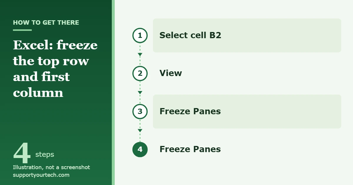
To freeze the top row and the first column in Excel at the same time, select cell B2, open the View tab, select Freeze Panes, and then choose Freeze Panes from the menu. Row 1 and column A now stay on screen while the rest of the worksheet scrolls.
Applies to: Excel for Microsoft 365, Excel 2024, Excel 2021, Excel 2019 and Excel 2016 on Windows, with separate sections for Excel for Mac and Excel for iPad and iPhone. Checked against Microsoft Support on October 6, 2026.
Why you select cell B2 first
Excel has three freeze commands, and only one of them can lock a row and a column together. Freeze Top Row locks row 1 only. Freeze First Column locks column A only. Neither one is the route Microsoft documents for holding both in place.
The third command, Freeze Panes, works from the cell you have selected. Microsoft describes the rule this way: Freeze Panes freezes the rows above and the columns left of the selected cell. Cell B2 has exactly one row above it (row 1) and one column to its left (column A), so it is the right starting point for this task.
Freeze the top row and first column in Excel for Windows
- Open the workbook and select the worksheet that you want to change.
- If you are typing in a cell, press Enter or Esc to finish editing first.
- Scroll to the top-left of the sheet so that row 1 and column A are both visible, then click cell B2. B2 is the cell in the second row of the second column.
- Select the View tab on the ribbon.
- Select Freeze Panes. A short menu opens.
- Select Freeze Panes in that menu. The menu closes and the freeze is applied.
- Scroll down and then to the right. Row 1 should stay at the top and column A should stay at the left the whole time.
Microsoft’s own instructions for this are on its Freeze panes to lock rows and columns support page.
Use the keyboard to reach Freeze Panes
You can open the same menu without the mouse. Select cell B2, then press Alt to show Key Tips, the small letters that appear next to each ribbon tab and command. Press Alt+W to open the View tab, and then press the letters shown on Freeze Panes and on the menu option you want. Because Excel displays the letters on screen, you do not have to memorize the sequence.
Freeze the top row and first column in Excel for Mac
Excel for Mac puts the freeze buttons directly on the View tab, so the path is one click shorter.
- Open the worksheet and select cell B2.
- Select the View tab.
- Select Freeze Panes.
- Scroll down and to the right to check that row 1 and column A stay in place.
If the freeze buttons are grayed out on a Mac, Microsoft’s instructions say to select Normal on the View tab first, then try again.
Freeze panes in Excel for iPad and iPhone
The mobile apps use the same rule: what you select decides what gets frozen.
- iPad: make your selection, then tap View > Freeze Panes > Freeze Panes.
- iPhone: make your selection, tap the ellipsis (…) button to open the ribbon, switch from Home to View, scroll down, and tap Freeze Panes.
To remove the freeze on either device, go back to View > Freeze Panes and clear the selected options.
How to confirm it worked
Scrolling is the real test, but there is also a visual cue. Microsoft notes that whenever rows and columns are frozen, the border below the last frozen row and to the right of the last frozen column appears a little thicker or darker than the other gridlines. After freezing at B2, look for that line under row 1 and to the right of column A.
If only one of the two stays put, the wrong cell was selected or one of the single-purpose commands was used. Unfreeze the sheet and repeat the steps from cell B2.
Unfreeze the row and column
- Select the View tab.
- Select Freeze Panes.
- Select Unfreeze Panes.
On a Mac, select Unfreeze Panes directly on the View tab. Unfreezing changes only what stays on screen. It does not delete or move any data.
Freeze more than one row or column
The same rule scales up. Pick the cell that sits just below the last row and just to the right of the last column you want to keep, then use View > Freeze Panes > Freeze Panes.
| You want to keep visible | Select this cell first |
|---|---|
| Row 1 and column A | B2 |
| Rows 1 and 2, and column A | B3 |
| Rows 1 and 2, and columns A and B | C3 |
| Rows 1 to 4, and columns A to C | D5 |
If you need columns only, select the whole column to the right of the ones you want to lock instead of a single cell. Our guide on how to freeze multiple columns in Excel walks through that version.
Troubleshooting
The sheet already has frozen panes
Clear the existing freeze before setting a new one. Go to View > Freeze Panes > Unfreeze Panes, click cell B2, and then choose View > Freeze Panes > Freeze Panes.
More rows or columns are frozen than you wanted
Excel freezes everything above and to the left of the selected cell, so selecting something like D10 locks nine rows and three columns. Unfreeze, scroll back to the top-left corner, select B2, and freeze again.
The freeze command is not available
Finish any cell edit by pressing Enter or Esc. If you are in a page-oriented view, go to View > Normal and try again.
There is no View tab
Microsoft says that if you do not see the View tab, you are probably using Excel Starter, which does not support every feature. In that case the freeze commands may not be available in your copy of Excel.
You want two scrolling areas rather than locked headings
That is a different feature. Select a cell and go to View > Window > Split to divide the sheet into panes that scroll separately. Select Split again to remove it.
Frequently asked questions
Can I use Freeze Top Row and then Freeze First Column?
That is not the method Microsoft documents. Its instructions for locking both are to select cell B2 and use Freeze Panes, which sets the row and the column in one action.
Do frozen panes print on every page?
No. Freezing only affects what you see while scrolling. To repeat headings on printed pages, open the Page Layout tab, select Print Titles, and on the Sheet tab fill in Rows to repeat at top (for example $1:$1) and Columns to repeat at left.
Does freezing change or protect my data?
No. Freezing only controls which rows and columns stay visible while you scroll. It is not a way to lock cells against editing.
What if my headings are not in row 1 or column A?
Select the cell just below your heading row and just to the right of your label column. Every row above it and every column to its left will be frozen, including any blank or title rows at the top.
With the headings locked, the next useful step for a long sheet is to set Print Titles so the same row and column also repeat on paper. If you only ever need the header row, see how to freeze the top row in Excel.
Related: how to unlock the cursor in Excel.
Related: how to highlight the active cell in Excel.

Matt Jacobs has been working as an IT consultant for small businesses since receiving his Master’s degree in 2003. While he still does some consulting work, his primary focus now is on creating technology support content for SupportYourTech.com.
His work can be found on many websites and focuses on topics such as Microsoft Office, Apple devices, Android devices, Photoshop, and more.