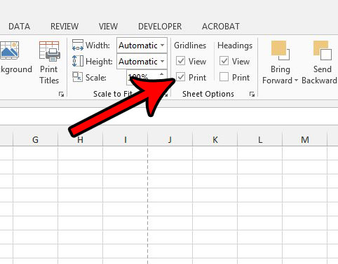
You might be interested in learning how to print gridlines in Excel 2013 if you have printed out a document and found it difficult to read because all of the data seemed to group together.
The lines separating the cells on your spreadsheet, called gridlines, and a very important factor in making the spreadsheet easier to read on your computer.
But those lines don’t print by default, so you need to adjust a setting to print gridlines in Excel 2013.
If you need to print cells that don’t have data in them, then our how to print empty gridlines in Excel tutorial will show you how.
Step 1: Open the spreadsheet in Excel 2013.
Step 2: Click the Page Layout tab at the top of the window.

Step 3: Check the box to the left of Print under Gridlines in the Sheet Options section of the ribbon.

Now that you know how to print gridlines in Excel 2013, you can make it much easier for other people to read the data in the spreadsheets that you print.
Another helpful print setting that you might want to use involves repeating a row at the top of every page in Excel 2013. This will make it much simpler for readers to identify the information contained within your cells.

Matt Jacobs has been working as an IT consultant for small businesses since receiving his Master’s degree in 2003. While he still does some consulting work, his primary focus now is on creating technology support content for SupportYourTech.com.
His work can be found on many websites and focuses on topics such as Microsoft Office, Apple devices, Android devices, Photoshop, and more.