How to Convert a Number to Text in Excel

Last updated on November 11th, 2026 at 06:05 pm

Excel’s =TEXT(A2,"0") formula turns A2’s number into text that looks the same; type it in an empty cell and press Enter. Before typing numbers, select the cells and choose Text from the Number Format drop-down on the Home tab, or start one entry with an apostrophe, like ‘02134.

That covers Microsoft 365 on Windows or Mac and Excel 2016 through 2024; TEXT behaves the same in Excel for the web (see Microsoft’s TEXT function reference).

When you want a number stored as text

Excel treats anything that looks like a number as a number. That’s what you want for prices and quantities, but it causes trouble with values that are really labels:

• ZIP codes and product codes with leading zeros. Type 02134 into a normal cell and Excel stores 2134.
• Long ID numbers. Excel keeps only 15 digits of precision for numbers, so a 16-digit card or account number has its last digit changed to zero.
• Phone numbers and part numbers that you’ll never add up, but need to match exactly in a lookup.
• Labels and sentences built with a formula, where a raw number would lose its currency sign or commas.

The catch: text doesn’t calculate. SUM skips text values, so a column of converted numbers adds up to 0. Keep anything you need to total as a real number, and change only how it looks with Excel’s number formats. If the value still needs to calculate, keep it numeric and apply the Comma Style format instead of converting it to text.

Is converting a number to text the same as writing it out in words?

No. Converting to text keeps the digits (1250 becomes the text “1250”). Spelling it out as “one thousand two hundred fifty” needs a different approach, explained in converting numbers to words in Excel.

Pick the right method

Your situation	Use this	Changes the original cell?
You’re about to type or paste values	Format the cells as Text first	Yes (only new entries)
Just a few values	Type an apostrophe first	Yes
A whole column of existing numbers	Text to Columns	Yes, in place
You need a specific look (zeros, commas, currency, dates)	TEXT function	No, result goes in a new cell
You need the plain value as text, no formatting	&”” or VALUETOTEXT	No, result goes in a new cell

Method 1: Format cells as Text before you type

This is the best choice for data entry, such as a column of ZIP codes or employee IDs you’re about to fill in.

1. Select the empty cells or the whole column (click the column letter).
2. On the Home tab, in the Number group, click the arrow next to the Number Format box (it usually says General) and choose Text. It’s near the bottom of the list. You can also press Ctrl + 1 (Command + 1 on a Mac), choose Text in the Category list and click OK.

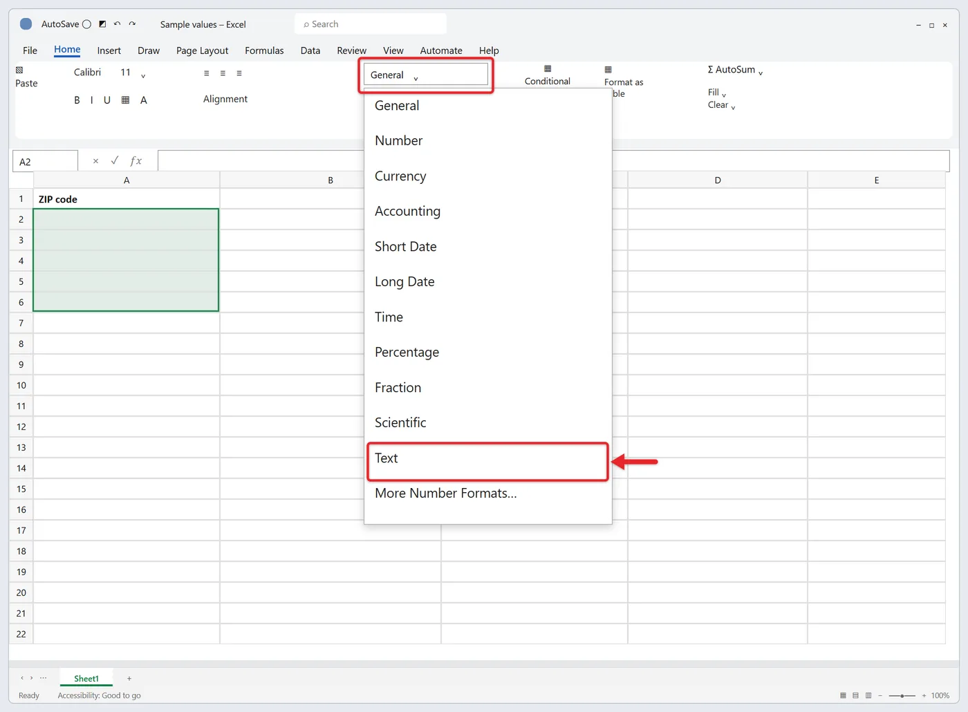
3. Type or paste your values. Leading zeros stay, and long IDs keep every digit.

Expect the entries to sit on the left side of the cell (text’s default alignment) and, in many cases, a small green triangle in the corner. That triangle is Excel’s “Number Stored as Text” check, not an error in your data.

Important: formatting cells that already hold numbers doesn’t convert those numbers. The cell shows the Text format, but the value is still a number until you edit it (press F2, then Enter). Digits Excel already dropped, like a leading zero or the 16th digit, don’t come back. For existing data, use Method 3 or Method 4.

Can I convert a whole column with one formula?

In Excel for Microsoft 365, Excel 2021 and Excel 2024, a formula like =TEXT(A2:A100,"00000") spills the results down the column automatically. In older versions, enter the formula in the first row and drag the fill handle down.

Method 2: Type an apostrophe first

For a one-off entry, type an apostrophe before the number: ‘00123. The apostrophe tells Excel to store what follows as text. It doesn’t appear in the cell or on a printout, only in the formula bar when the cell is selected.

This is the quickest fix for a handful of cells. For hundreds of rows, Method 1 or Method 3 saves a lot of typing. Like Method 1, it only protects what you type now; adding an apostrophe to a long number that Excel already rounded won’t restore the lost digits.

Method 3: Convert an existing column with Text to Columns

Text to Columns is designed to split data, but its last step can also convert a column to text in place, with no helper column or formulas.

1. Select the cells in one column (Text to Columns works on one column at a time).
2. On the Data tab, click Text to Columns. The Convert Text to Columns Wizard opens.
3. Leave Delimited selected and click Next.
4. Clear every box under Delimiters so nothing gets split, then click Next.
5. Under Column data format, choose Text. Check that Destination shows your first selected cell, then click Finish.

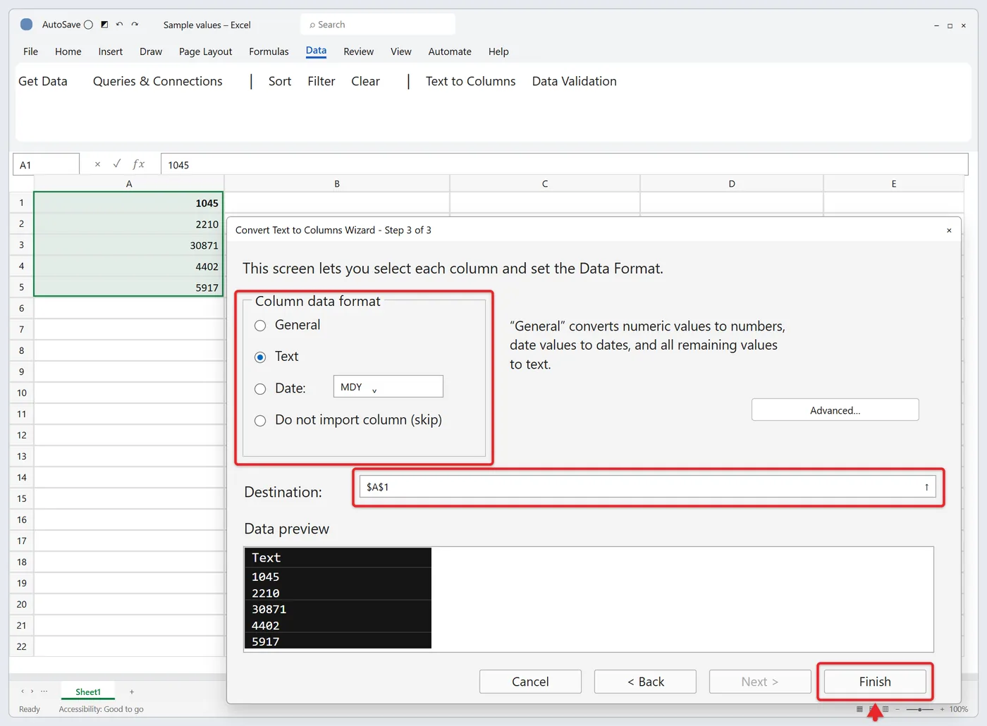
The values jump to the left side of their cells and the column is now formatted as Text. If a number shows in scientific notation (like 1.23E+15) before you start, widen the column or fix the E+ display first, so you can confirm what Excel actually stored.

These steps are for the Excel desktop apps. If you don’t see the Column data format options in Excel for the web, use the TEXT function below instead.

Do these methods work in Google Sheets?

The apostrophe and the TEXT function work there too. Instead of a Text format, Google Sheets uses Format > Number > Plain text.

Method 4: Use the TEXT function

TEXT turns a number into text in exactly the format you specify:

=TEXT(value, format_text)

The value is the number or cell, and format_text is a format code in double quotes. The original cell stays untouched, which is why Microsoft recommends keeping the number in one cell and the TEXT result in another.

Common format codes

Each example uses the sample value shown in the third column:

Goal	Formula	Value in A2	Result
Whole number, no formatting	=TEXT(A2,"0")	1234.5	1235
Thousands separator, 2 decimals	=TEXT(A2,"#,##0.00")	1234.5	1,234.50
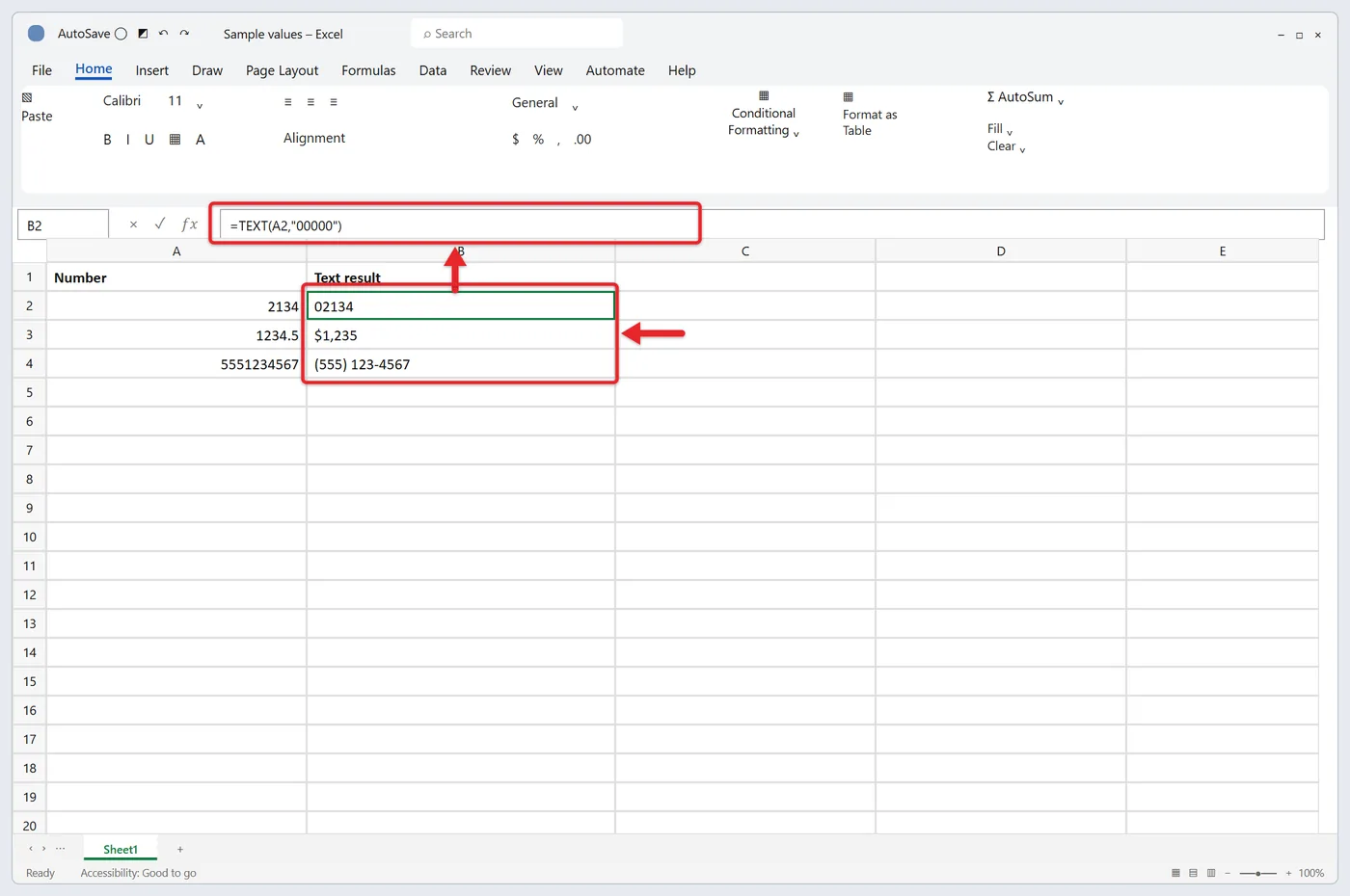
Currency, no cents	=TEXT(A2,"$#,##0")	1234.5	$1,235
Five-digit ZIP code	=TEXT(A2,"00000")	2134	02134
Pad an ID to six digits	=TEXT(A2,"000000")	1234.5	001235
Phone number	=TEXT(A2,"(000) 000-0000")	5551234567	(555) 123-4567
Percentage	=TEXT(A2,"0.0%")	0.25	25.0%
Date	=TEXT(A2,"mmm d, yyyy")	10/27/2026	Oct 27, 2026
Day of the week	=TEXT(A2,"dddd")	10/27/2026	Tuesday

Notice that TEXT rounds: 1234.5 becomes 1235 with “0” or “$#,##0”. Add decimal places to the code (like “0.00”) if you need them. In a zero-padding code, the number of zeros is the total length you want, so “00000” always gives five characters for numbers up to five digits.

Not sure which code you need? Format a cell the way you like, press Ctrl + 1, choose Custom, and copy the code from the Type box into your formula, inside the quotes.

Put a formatted number inside a sentence

This is where TEXT really earns its keep. If B10 holds 48250, then ="Total sales: "&B10 returns “Total sales: 48250,” because joining strips the cell’s formatting. Wrap the number in TEXT instead:

="Total sales: "&TEXT(B10,"$#,##0") returns Total sales: $48,250.

The & operator is one of several ways to combine text and cells with concatenation; TEXT works the same way inside CONCAT or TEXTJOIN.

Why does TEXT give me a #NAME? error?

Most often the format code is missing its double quotes. =TEXT(A2,mmm) fails because Excel reads mmm as a name; =TEXT(A2,"mmm") works.

Method 5: Join an empty string, or use VALUETOTEXT

When you want the value as text without picking a format, join it to an empty string: =A2&"". If A2 holds 1234.5, the result is the text “1234.5”. This is handy for lookup keys when one list stores IDs as numbers and another stores them as text.

In Excel for Microsoft 365 and Excel 2021 or later, =VALUETOTEXT(A2) does the same job and also handles logical values and errors. An optional second argument of 1 gives the “strict” format, which wraps text values in quotation marks so the result could be pasted back into a formula. See Microsoft’s VALUETOTEXT page for the full list of outputs.

One trap with both: they return the stored value, not what you see. A cell showing $1,234.50 becomes “1234.5”, and a date becomes its serial number (October 27, 2026 becomes “46322”). Use TEXT when the look matters.

Keep the text and remove the formulas

Methods 4 and 5 leave formulas in your sheet. To replace them with fixed text:

1. Select the formula cells and press Ctrl + C.
2. Select where the text should go (the same cells, or over the original numbers).
3. On the Home tab, click the arrow under Paste, and under Paste Values choose Values (the icon showing 123).

The cells now hold plain text, and you can delete the original number column if you no longer need it.

Stop imports from stripping zeros

Opening a CSV file by double-clicking it lets Excel guess the data types, and it guesses “number” for ZIP codes and IDs. Instead, use Data > From Text/CSV, click Transform Data, and set the ID column’s data type to Text in Power Query before loading. The steps are covered in more detail in importing a CSV file into Excel, and leading zeros in particular get a full walkthrough in how to stop Excel from removing leading zeros.

How to confirm the conversion worked

• Alignment: text sits on the left by default and numbers on the right (unless someone set the alignment manually).
• Status bar: select the cells. Numbers show Sum and Average at the bottom of the window; text cells show only Count.
• A formula check: =ISTEXT(A2) returns TRUE for text and FALSE for a number.

To undo right away, press Ctrl + Z. To undo later, convert the values back to numbers as shown next.

The reverse problem: numbers stored as text

Sometimes you get the opposite: imported numbers that are stuck as text, so SUM returns 0 and sorting puts 100 before 20. Microsoft’s guide to converting numbers stored as text covers these fixes:

• Convert to Number: select the cells, click the warning icon that appears next to them and choose Convert to Number. If you don’t see the icon, turn on Enable background error checking under File > Options > Formulas.
• VALUE: =VALUE(A2) turns the text “00042” into the number 42. Then paste the results as values.
• Math shortcut: =A2*1 or =--A2 also return 42 for “00042”.

Leading zeros vanish when text becomes a number, so convert only columns you actually calculate with.

Green triangles and missing leading zeros

• Green triangles everywhere. That’s the “Number Stored as Text” warning. If text is what you want, select the cells, click the warning icon and choose Ignore Error.
• Leading zeros still missing. The cells were set to Text after the numbers were typed. Re-enter the values, or rebuild the zeros with =TEXT(A2,"00000") using the right number of zeros.
• Long numbers end in 0. Excel had already stored them as numbers and kept only 15 digits. Format the column as Text, then type or paste the original values again from the source.
• Totals show 0. Your SUM range contains text. Keep a numeric copy for math, or convert back with VALUE.
• VLOOKUP or XLOOKUP returns #N/A. The lookup value is a number and the list holds text (or the other way around). Match the types with TEXT(D2,"0") or D2&"" inside the lookup.
• The format code is ignored or gives odd results. Codes follow your regional settings. Some locales use a comma for decimals and a period or space for thousands, and month codes can differ by language.
• The formula shows as text instead of a result. The cell was formatted as Text before you typed the formula. Set it to General, then press F2 and Enter.

For data you’re typing, set the column to Text first; for data you already have, reach for Text to Columns or TEXT. Once your codes are stored as text, you can pull out pieces of them, such as a region prefix, with the LEFT function.