To edit a pivot table in Excel, click any cell inside it so the PivotTable Fields list opens on the right, then drag fields between the Filters, Columns, Rows and Values boxes. Change how numbers are calculated with Value Field Settings, update the source range with PivotTable Analyze > Change Data Source, and change the look on the Design tab. Each is covered step by step below.
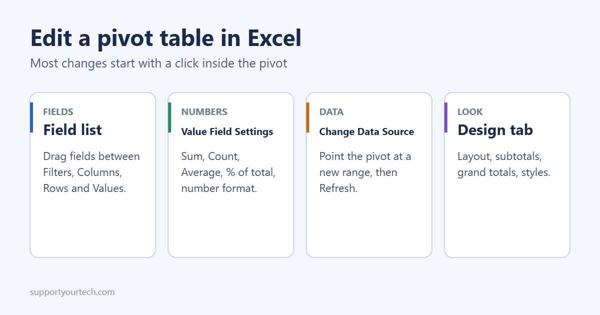
If the field list or the PivotTable tabs don’t appear, see how to find a pivot table in Excel.
Add, remove and move fields
- Add a field: tick its box in the field list, or drag it into one of the four areas.
- Remove a field: untick it, or drag it out of the area box and drop it on the list.
- Move a field: drag it from Rows to Columns, for example, to turn the table on its side.
- Change the order: drag fields up or down within Rows to change which grouping comes first.
| Area | What it does |
|---|---|
| Filters | Adds a drop-down above the pivot to filter the whole table |
| Columns | Spreads values across the top |
| Rows | Lists values down the left side |
| Values | The numbers being summed, counted or averaged |
Tick Defer Layout Update at the bottom of the field list if the pivot is large and slow. Excel then waits until you click Update.
Change the calculation
- In the Values area, click the field (for example “Sum of Sales”) and choose Value Field Settings.
- On Summarize Values By, choose Sum, Count, Average, Max, Min or another function.
- On Show Values As, choose options like % of Grand Total, % of Column Total or Running Total In.
- Click Number Format to set currency, decimals or percentages for the whole field.
- Change Custom Name to rename the column, then click OK.
If a number field shows “Count of” instead of “Sum of”, the source column contains blanks or text. Change it to Sum here, and clean up the source data to stop it happening again.
Rename fields and items
Click a header or label in the pivot and type a new name. A field can’t have exactly the same name as a source column, so to rename “Sum of Sales” to “Sales”, type “Sales ” with a trailing space.
Change or expand the source data
- Click inside the pivot.
- Go to PivotTable Analyze > Change Data Source.
- Select the new range, including headers, and click OK.
To stop doing this every time you add rows, format the source data as a table with Ctrl + T before creating the pivot. The pivot then uses the table name and grows with it automatically.
Refresh after the data changes
Pivot tables don’t update by themselves. After editing the source, click inside the pivot and press Alt + F5, or go to PivotTable Analyze > Refresh. Ctrl + Alt + F5 refreshes every pivot and data connection in the workbook. To refresh automatically when the file opens, go to PivotTable Analyze > Options > Data and tick Refresh data when opening the file.
Filter, sort and group
- Filter: click the arrow next to Row Labels or Column Labels and untick items, or use Label and Value Filters such as Top 10.
- Slicers: PivotTable Analyze > Insert Slicer adds clickable filter buttons.
- Sort: right-click a value and choose Sort > Largest to Smallest.
- Group dates: right-click a date and choose Group, then pick Months, Quarters and Years.
- Group numbers: right-click a number in Rows, choose Group, and set a range size such as 10 for age bands.
Change the layout and design
| Design tab option | Choices |
|---|---|
| Report Layout | Compact, Outline or Tabular form, and Repeat All Item Labels |
| Subtotals | Show at top, at bottom, or not at all |
| Grand Totals | On or off for rows and columns |
| Blank Rows | Insert a blank line after each item |
| PivotTable Styles | Colors and banding |
Tabular Form with Repeat All Item Labels is the easiest layout to copy into another sheet as plain data.
Stop column widths from changing
Right-click the pivot, choose PivotTable Options, and untick Autofit column widths on update. In the same dialog, set For empty cells show to 0 to replace blanks.
Add a calculated field
To create a column that doesn’t exist in the source, such as profit from sales and cost, go to PivotTable Analyze > Fields, Items & Sets > Calculated Field. Name it, enter a formula like =Sales-Cost using the field list, and click Add.
Troubleshooting
“We can’t change this part of the PivotTable”
You can’t type over numbers in a pivot. Change the source data and refresh instead, or copy the pivot and use Paste Values if you need an editable copy.
New rows don’t appear after refreshing
The source range doesn’t include them. Use Change Data Source, or convert the source to a table.
“The PivotTable field name is not valid”
A column in the source has a blank header. Give every column a heading, then refresh.
Mac and Excel for the web
On a Mac the tabs are called PivotTable Analyze and Design, and Value Field Settings opens from the small i button next to a field. Excel for the web supports most of the same edits from the field pane on the right, including Value Field Settings and refresh.
Related guides
- How to make a pivot table in Excel
- How to refresh a pivot table
- How to insert a slicer
- How to use PIVOTBY for a formula-based pivot
Summary
- Click inside the pivot to open the field list.
- Drag fields between Filters, Columns, Rows and Values.
- Use Value Field Settings to change Sum to Count or Average.
- Use Change Data Source and Refresh after the data changes.
- Use the Design tab for layout, totals and style.

Matt Jacobs has been working as an IT consultant for small businesses since receiving his Master’s degree in 2003. While he still does some consulting work, his primary focus now is on creating technology support content for SupportYourTech.com.
His work can be found on many websites and focuses on topics such as Microsoft Office, Apple devices, Android devices, Photoshop, and more.