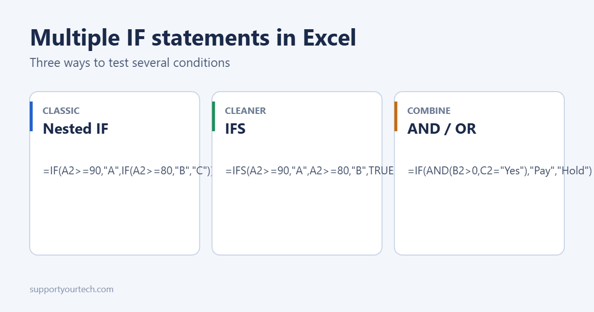
To do multiple IF statements in Excel, put one IF inside another: =IF(A2>=90,"A",IF(A2>=80,"B","C")). Excel checks the first condition, and only if it’s false moves to the next IF. In Excel 2019 and later, the IFS function does the same job with less nesting: =IFS(A2>=90,"A",A2>=80,"B",TRUE,"C"). If you need several conditions to be true at once, combine IF with AND or OR instead. Examples of each are below.
How a nested IF works
The IF function has three parts: =IF(test, value_if_true, value_if_false). In a nested IF, the value_if_false part is another IF. Here’s a grading example for a score in A2:
=IF(A2>=90,"A",IF(A2>=80,"B",IF(A2>=70,"C",IF(A2>=60,"D","F"))))
- Is A2 at least 90? If yes, return “A” and stop.
- If not, is it at least 80? If yes, return “B”.
- If not, check 70, then 60.
- If none are true, return “F”.
Order matters. Test from the highest threshold down (or lowest up). If you checked A2>=60 first, a score of 95 would get a “D”, because Excel stops at the first true test.
Count the closing brackets: one for each IF. Excel highlights matching pairs in color as you type, which helps.
The IFS function (Excel 2019 and later)
IFS lists test and result pairs without nesting:
=IFS(A2>=90,"A",A2>=80,"B",A2>=70,"C",A2>=60,"D",TRUE,"F")
The final TRUE,"F" acts as “everything else”. Without it, IFS returns #N/A when no condition is met. IFS is available in Excel for Microsoft 365, Excel 2019 and later, and Excel for the web. Files using it show #NAME? in Excel 2016 and older.
Test several conditions at once with AND and OR
Nesting is for “if this, else if that”. When you need “if this and that”, use AND or OR inside one IF:
| Goal | Formula |
|---|---|
| Both must be true | =IF(AND(B2>=1000,C2="Paid"),"Bonus","No bonus") |
| Either can be true | =IF(OR(D2="VIP",E2>5),"Priority","Standard") |
| Not equal | =IF(NOT(F2="Closed"),"Follow up","") |
| Mixed | =IF(AND(B2>0,OR(C2="East",C2="West")),"Ship","Hold") |
Return a number instead of text
Results don’t have to be text. This calculates commission at different rates based on sales in B2:
=IF(B2>=50000,B2*0.1,IF(B2>=20000,B2*0.07,B2*0.05))
Leave numbers out of quotes, or Excel treats them as text and they won’t add up.
Build a nested IF step by step
Long nested formulas are easier to get right if you build them one level at a time:
- Write the simplest version first, with one test:
=IF(A2>=90,"A","other"). Copy it down and check the results. - Replace
"other"with the next IF:=IF(A2>=90,"A",IF(A2>=80,"B","other")). Check again. - Repeat until every band is covered, then replace the last
"other"with your final fallback value.
To make long formulas readable, press Alt + Enter in the formula bar to put each IF on its own line. Excel ignores the line breaks when it calculates. Widen the formula bar with the arrow at its right end if you can’t see the whole formula.
Worked example: shipping cost
Say an order weight is in B2 (kg) and the destination is in C2. Domestic orders cost $5 under 1 kg, $9 up to 5 kg and $15 above that. International orders cost double. One formula handles both:
=IF(C2="Domestic",1,2)*IF(B2<1,5,IF(B2<=5,9,15))
The first IF picks the multiplier, and the nested IF picks the base price. Splitting the logic like this keeps each part short, and you can change a price without untangling the whole formula. If the prices change often, move them to cells and refer to those instead, with absolute references such as $F$2 so the formula copies down correctly.
When to use something other than IF
| Situation | Better choice |
|---|---|
| Many fixed matches (codes to names) | SWITCH or a lookup table with XLOOKUP |
| Score bands or price tiers | A lookup table with XLOOKUP(A2,Bands,Grades,,-1) |
| Counting or summing based on a condition | COUNTIF, SUMIF or SUMIFS |
| Coloring cells by condition | Conditional formatting |
A lookup table is easier to update than a long nested IF. Put thresholds in one column and results in the next, sorted ascending, and change the table instead of the formula. For example, =SWITCH(A2,"N","North","S","South","E","East","W","West","Unknown") replaces four nested IFs for exact matches.
See how to categorize data in Excel, how to use SUMIF and how to make a cell turn a color with a formula.
Common errors
“You’ve entered too few arguments” or a formula error
A comma or bracket is missing. Click in the formula bar, and Excel shows the argument tooltip for the IF you’re in. Check that every IF has a test, a true value and a false value.
The result is always the same
The tests are in the wrong order, or the cell holds text that looks like a number. Check with =ISNUMBER(A2).
#NAME?
Text results are missing quotes, or the version of Excel doesn’t support IFS. Wrap text in double quotes, or switch to nested IF.
Blank cells give the wrong result
A blank cell counts as 0. Add a first check: =IF(A2="","",IF(A2>=90,"A",...)).
Frequently asked questions
How many IFs can I nest?
Up to 64 in current versions. In practice, more than three or four becomes hard to read, so switch to IFS or a lookup table.
Can I use IF with dates?
Yes. Compare with the DATE function: =IF(A2<DATE(2026,1,1),"Old","New"), or with TODAY(): =IF(A2<TODAY(),"Overdue","").
Summary
- Nested IF:
=IF(test1,result1,IF(test2,result2,else)), highest threshold first. - IFS:
=IFS(test1,result1,test2,result2,TRUE,else)in Excel 2019 and later. - AND and OR: several conditions in one test.
- Lookup table or SWITCH: when the list of conditions gets long.
Related: enable iterative calculation in Excel.

Matt Jacobs has been working as an IT consultant for small businesses since receiving his Master’s degree in 2003. While he still does some consulting work, his primary focus now is on creating technology support content for SupportYourTech.com.
His work can be found on many websites and focuses on topics such as Microsoft Office, Apple devices, Android devices, Photoshop, and more.