How to Calculate Percentage Change in Excel

To calculate percentage change in Excel, put the old value in one cell and the new value in another, then type =(new-old)/old in a third cell, for example =(C2-B2)/B2. Press Enter, then select Home > Percent Style (the % button in the Number group) to show the result as a percentage. A positive result is an increase and a negative result is a decrease.

Applies to: Excel for Microsoft 365 (Windows, Mac and the web), Excel 2024, Excel 2021, Excel 2019 and Excel 2016. The one-formula spill option needs Microsoft 365, Excel 2024 or Excel 2021. The formulas follow Microsoft’s article on calculating percentages.

The percentage change formula

Percentage change tells you how much a value grew or shrank compared with where it started. The formula is:

(new value - old value) / old value

The top part finds the amount of change. Dividing by the old value turns that amount into a share of the starting point. For example, if a store sold 1,250 bags of coffee beans last year and 1,400 this year, the change is 150 bags, and 150 divided by 1,250 is 0.12, or 12%.

A few things are worth knowing before you start:

• Always divide by the old value. Dividing by the new value answers a different question and gives a different number. Going from 1,250 to 1,400 is a 12% increase, but going from 1,400 back to 1,250 is a 10.7% decrease, because the starting point changed.
• The parentheses matter. Excel divides before it subtracts. Without parentheses, =C2-B2/B2 divides B2 by itself first and then subtracts 1 from C2, which is not what you want.
• There’s a shorter version. =C2/B2-1 gives exactly the same answer. Use whichever one is easier for you to read.
• Excel has no PERCENTCHANGE function. You build the result with a simple formula, which also means you can see exactly how it is calculated.
• Don’t multiply by 100. Excel stores 12% as 0.12. The Percent Style format does the multiplying for you when it displays the number.

How to calculate percentage change between two cells

The examples in this guide use a small sales sheet. Column A lists items, column B has 2025 Sales, column C has 2026 Sales, and column D will hold the % Change. Row 1 has the headers, and the data is in rows 2 to 7.

Row	Item (A)	2025 Sales (B)	2026 Sales (C)	% Change (D)
2	Coffee beans	1,250	1,400	12.0%
3	Pastries	860	731	-15.0%
4	Tea	640	672	5.0%
5	Gift cards	520	0	-100.0%
6	Sandwiches	300	300	0.0%
7	Mugs	0	75	#DIV/0! (see zero values)

1. Put the old and new values side by side. Type the starting values in column B and the newer values in column C. Make sure they are real numbers. If a cell shows a small green triangle in its corner or the numbers are left-aligned, they may be stored as text, which causes a #VALUE! error later.
2. Select the result cell. Click cell D2, next to the first pair of values.
3. Type the formula. Type =(C2-B2)/B2. You can type the cell addresses or click the cells while you build the formula. As you type, Excel outlines B2 and C2 in color so you can check that you picked the right cells.
4. Press Enter. D2 shows 0.12. That’s the correct answer. It just isn’t formatted as a percentage yet.

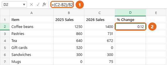
If you only need a quick answer and don’t want to use cells, you can type the numbers straight into the formula, such as =(1400-1250)/1250. Cell references are better for real work, because the result updates as soon as either value changes.

Show the result as a percentage

Formatting changes how the number looks, not the value Excel stores. D2 still holds 0.12 after you format it as 12%.

1. Select the result cells. Click D2, or drag over all the cells in column D that hold results.
2. Apply Percent Style. On the Home tab, select Percent Style (the % button) in the Number group. On Windows, you can press Ctrl+Shift+% instead. D2 now shows 12%.
3. Add decimal places if you need them. Percent Style shows whole percentages only, so 8.74% appears as 9%. Select Increase Decimal in the same group once to show one decimal place, such as 12.0% or 8.7%. Select Decrease Decimal to remove places.

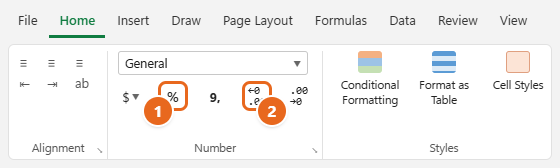
You can also set the exact number of decimal places in one step. Press Ctrl+1 (on a Mac, Command+1) to open Format Cells, select Percentage on the Number tab, set Decimal places, and select OK. Other display options are covered in changing the number format in Excel.

Show a plus sign or color for increases and decreases

Excel puts a minus sign in front of decreases but shows nothing in front of increases. If you’d like every result to show its direction, use a custom number format:

1. Select the result cells and press Ctrl+1.
2. On the Number tab, select Custom.
3. In the Type box, enter +0.0%;-0.0%;0.0% and select OK.

The three parts, separated by semicolons, control positive numbers, negative numbers and zero. 12% now shows as +12.0% and a 15% drop shows as -15.0%. To color them too, use [Blue]+0.0%;[Red]-0.0%;0.0%. If you’d rather use fill colors or icons, conditional formatting can do that, as explained in coloring cells based on their value.

Calculate percentage change for a whole column

Once D2 works, you don’t need to type the formula again for each row.

1. Select D2. A small square, the fill handle, appears in the bottom-right corner of the cell.
2. Copy the formula down. Double-click the fill handle to fill down to the last row of your data, or drag it down to D7. Excel adjusts the references for each row, so D3 contains =(C3-B3)/B3, D4 contains =(C4-B4)/B4, and so on.
3. Check the results. With the sample data, you’ll see 12.0%, -15.0%, 5.0%, -100.0% and 0.0%, plus a #DIV/0! error for Mugs, which had no sales in 2025. The next sections explain how to deal with that.

One formula for the whole column: In Excel for Microsoft 365, Excel 2024 and Excel 2021, you can type =(C2:C7-B2:B7)/B2:B7 in D2 instead. The results spill down into D3:D7 automatically. If you see a #SPILL! error, something is already typed in the cells below, so clear them.

Find the change for the total, not the average

To see how the whole store did, don’t average the percentages in column D. Add the old values and the new values first, then use the same formula on the totals. With the sample data, total sales went from 3,570 to 3,178, so =(SUM(C2:C7)-SUM(B2:B7))/SUM(B2:B7) returns -11.0%. Averaging the five row results instead gives -19.6%, which overstates the drop because a small item like gift cards counts as much as coffee beans.

Month-over-month and change from a fixed start

When your values are listed in time order down one column, the old value is the row above or a single starting row. Suppose column A lists months from January in row 2 to June in row 7, and column B has revenue of 4,000, 4,400, 4,180, 4,598, 5,000 and 4,750.

Change from the previous period

1. Click C3. Leave C2 empty, because January has no earlier month to compare with.
2. Type =(B3-B2)/B2 and press Enter.
3. Fill the formula down to C7 and apply Percent Style with one decimal place.

February shows 10.0%, March -5.0%, April 10.0%, May 8.7% and June -5.0%. The same pattern gives year-over-year change when each row is a year.

Change from a fixed starting point

To compare every month with January instead, lock the starting cell with dollar signs so it doesn’t move when you copy the formula:

1. Click D3 and type =(B3-$B$2)/$B$2. While typing, you can click B2 in the formula and press F4 to add the dollar signs.
2. Press Enter and fill down to D7.

Every row now divides by January’s 4,000. June shows 18.8% even though it dropped 5.0% from May. If dollar signs are new to you, absolute cell references in Excel explains how they work.

When the old value is zero or blank

Percentage change is measured against the old value, so it can’t be calculated when the old value is zero. Going from 0 to 75 is not a 75% increase or a 100% increase. Mathematically, there is no percentage at all, which is why Excel returns #DIV/0!.

Some guides suggest hiding the error with =IFERROR((C2-B2)/B2,0) or forcing the answer to 100%. Both make the result look like a real number when it isn’t. A row that went from 0 to 75 would show 0% (no change) or 100%, and anyone reading the sheet would draw the wrong conclusion. IFERROR also hides other errors, such as a typo or a text value, that you’d want to see. A clear label is safer.

Warning: Excel treats an empty cell as zero in a formula. A blank old value causes #DIV/0!, and a blank new value is worse: =(C2-B2)/B2 quietly returns -100%, as if sales had dropped to nothing. This often happens when you set up formulas for months that haven’t happened yet.

To handle both cases:

1. Click E2 and type =IF(B2=0,"n/a",(C2-B2)/B2). The IF function checks whether the old value is 0 (a blank cell counts as 0 too). If it is, the cell shows n/a. Otherwise, it calculates the normal percentage change.
2. Press Enter, fill the formula down, and apply Percent Style. The Mugs row now shows n/a instead of an error, and every other row matches column D.
3. If some rows may not have a new value yet, use this version instead: =IF(OR(B2="",C2=""),"",IF(B2=0,"n/a",(C2-B2)/B2)). It leaves the cell blank until both values are entered.

The screenshot below uses the combined version with ABS from the next section, =IF(B7=0,"n/a",(C7-B7)/ABS(B7)). For positive starting values like these, it gives exactly the same results.

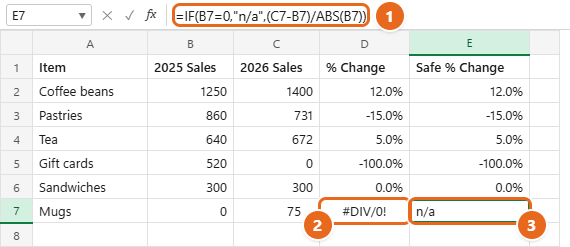
You can replace “n/a” with any label that suits your report, such as “New” for a product that had no sales last year. If you’d rather show the change in units for those rows, use =IF(B2=0,C2-B2,(C2-B2)/B2), but remember that column then mixes counts and percentages, so label it clearly.

A drop to zero is different. Going from 520 to 0 is a real -100% change, and the basic formula handles it correctly.

When the old value is negative

Negative numbers show up in profit, cash flow, temperatures and account balances. The basic formula gives the right size of change when the old value is negative, but the wrong sign, because dividing by a negative number flips the result. The fix is to divide by the absolute value of the old number with the ABS function, which drops the minus sign:

=(C2-B2)/ABS(B2)

Here’s how the two formulas compare on quarterly profit figures:

Region	Q1 profit (B)	Q2 profit (C)	=(C2-B2)/B2	=(C2-B2)/ABS(B2)
North	-500	-200	-60.0% (wrong direction)	60.0%
South	-500	250	-150.0% (wrong direction)	150.0%
East	400	-100	-125.0%	-125.0%
West	-200	-500	150.0% (wrong direction)	-150.0%

North’s loss shrank from 500 to 200, which is an improvement, so the result should be positive. The ABS version gets that right. When the old value is positive, as in the East row, both formulas give the same answer, so you can safely use the ABS version for the whole column. To handle zeros as well, combine the two fixes: =IF(B2=0,"n/a",(C2-B2)/ABS(B2)).

Be careful when the sign flips. Even with ABS, a change from a loss to a profit is hard to read as a percentage. A region that went from -300 to 300 shows 200%, while one that went from -400 to 300 shows 175%, even though the second region improved by more dollars. Many financial reports show “NM” (not meaningful) in these cases and report the change in dollars instead. To do that, use =IF(B2=0,"n/a",IF(B2*C2<0,"NM",(C2-B2)/ABS(B2))). The product of the two values is negative only when one is positive and the other is negative.

Related calculations: work backward, percentage points and growth rates

Find the new value from a percentage change

If you know the old value and the percentage change, multiply by 1 plus the change. With the old value in B2 and the change in D2, use =B2*(1+D2). For example, 1,250 increased by 12% is 1,400. A negative change works the same way: 860 with a -15% change gives 731. More examples, such as adding a fixed 10% to a whole column, are in multiplying by a percentage in Excel.

Find the old value from the new value

To work backward, divide by 1 plus the change: =C2/(1+D2). 1,400 divided by 1.12 returns 1,250. Don’t subtract the percentage from the new value instead. 1,400 minus 12% is 1,232, not 1,250, because the 12% was measured from the smaller starting number.

Percentage change vs. percentage points

When the values are already percentages, be clear about which difference you mean. If an email open rate rises from 20% to 25%, it went up 5 percentage points (=C2-B2), but the percentage change is 25% (=(C2-B2)/B2). Both are correct. They just answer different questions, so label your column.

Percentage change vs. percentage difference

Percentage change needs a clear “before” and “after.” When you compare two values with no natural order, such as quotes of $450 and $500 from two suppliers, use percentage difference, which compares the gap with the average of the two: =ABS(C2-B2)/AVERAGE(B2,C2). For those quotes it returns 10.5%, whichever order you put them in.

Average growth per period

If sales grew from 1,000 to 1,331 over three years, the total change is 33.1%. Dividing that by 3 (11.0% a year) overstates the yearly rate, because each year’s growth builds on the last. The compound annual growth rate is =(C2/B2)^(1/3)-1, which returns 10.0%. Excel also has a built-in function for this, RRI, which takes the number of periods, the starting value and the ending value: =RRI(3,1000,1331) also returns 10.0%. For growth driven by an interest rate, use the formulas for compound interest in Excel.

Troubleshooting

The result shows 0.12 instead of 12%

The formula is right. The cell just uses the General number format. Select the cell and apply Percent Style on the Home tab.

The result shows 1200% instead of 12%

The formula multiplies by 100 and the cell is also formatted as a percentage, so the value is scaled twice. Remove *100 from the formula and let the format handle it. If you really want a plain number like 12, keep *100 and change the format back to General or Number.

Small changes show as 0%

Percent Style rounds to whole numbers, so a 0.4% change displays as 0%. Select Increase Decimal until you can see it. The stored value was never rounded.

#DIV/0! error

The old value is 0 or the cell is blank. Check that the formula points to the right cell, then use the IF version from When the old value is zero or blank.

#VALUE! error

One of the cells contains text, such as “N/A”, a stray space, or a number stored as text. Retype the value, or select the cell, select the warning icon next to it and choose Convert to Number.

Increases show as negative numbers

The old and new cells are swapped. The new value goes first in the subtraction, and the old value goes in the denominator: =(new-old)/old. If both numbers are negative, see When the old value is negative.

Copied formulas give wrong results or #DIV/0! further down

If every row should compare with one starting cell, the reference to that cell needs dollar signs, such as $B$2. Without them, Excel moves the reference down a row each time you copy the formula, and it can end up pointing at an empty cell.

FAQ

What is the formula for percentage change in Excel?

Use =(new-old)/old, for example =(C2-B2)/B2 with the old value in B2 and the new value in C2. =C2/B2-1 gives the same result. Format the cell as a percentage to read it.

How do I calculate a percentage decrease in Excel?

Use the same formula. When the new value is smaller, the result is negative, such as -15%. If you want a positive number for a decrease, for example to report “sales fell 15%”, use =(B2-C2)/B2 or wrap the formula in ABS, but label the column so readers know it’s a decrease.

Is there a percentage change function in Excel?

No. Excel doesn’t have a dedicated function for percentage change between two values. The simple formula is the standard method, and it works in every version of Excel, including Excel for the web and Excel for Mac.

How do I calculate percentage change when the old value is 0?

You can’t, because a change from zero has no percentage. Use =IF(B2=0,"n/a",(C2-B2)/B2) to show a label instead of an error, and report the change in units if you need a number.

How do I handle negative numbers?

Divide by the absolute value of the old number: =(C2-B2)/ABS(B2). This keeps the sign correct, so an improvement from -500 to -200 shows as a positive 60%.

How do I get rid of the minus sign but keep the color?

Use a custom format such as 0.0%;[Red]0.0%. Negative results show in red without a minus sign, but the cell still holds a negative value, so formulas that use it still work correctly.

Does this work in Google Sheets?

Yes. The formula, the IF and ABS versions, and RRI all work the same way in Google Sheets. The formatting buttons are in a different place on the toolbar.

Once your percentage change column works, try the version with IF and ABS on your own data first, since it handles zeros and negative numbers in one formula. Then add color to the results so increases and decreases stand out at a glance.