How to Use IFERROR in Excel

To use IFERROR in Excel, wrap the formula that might fail like this: =IFERROR(formula, value_if_error). For example, =IFERROR(B2/C2,"No orders") shows the result of B2/C2 when it works and shows No orders instead of #DIV/0! when it doesn’t. Type it in a cell and press Enter, or select Formulas > Logical > IFERROR to fill it in with a dialog box.

Applies to: Excel for Microsoft 365 (Windows, Mac and the web), Excel 2024, Excel 2021, Excel 2019 and Excel 2016. Single-formula spilled results and XLOOKUP need Microsoft 365, Excel 2024 or Excel 2021. Function details match Microsoft’s IFERROR reference.

How IFERROR works

IFERROR checks one formula. If that formula produces an error, IFERROR shows a value you choose. If there’s no error, it shows the formula’s normal result. The syntax is:

=IFERROR(value, value_if_error)

• value is the formula or cell you want to check, such as B2/C2 or a VLOOKUP.
• value_if_error is what to show if value is an error. It can be text in double quotes, a number, an empty string (""), or another formula.

Both arguments are required. IFERROR catches these error types: #N/A, #VALUE!, #REF!, #DIV/0!, #NUM!, #NAME? and #NULL!. That catch-all behavior is both its strength and its biggest risk, as you’ll see in the examples.

IFERROR has been in Excel since Excel 2007, so a workbook that uses it opens correctly in any version you are likely to meet today.

Add IFERROR to a formula, step by step

The examples in this guide use a small store report. Column A has the store name, column B has total sales, column C has the number of orders, and column D calculates the average sale per order with =B2/C2.

Row	Store (A)	Sales (B)	Orders (C)	=B/C result (D)
2	Denver	$4,800	120	$40.00
3	Austin	$2,250	0	#DIV/0!
4	Boise	$3,600	80	$45.00
5	Tampa	$1,950	(empty)	#DIV/0!
6	Reno	$5,400	150	$36.00
7	Salem	$2,640	TBD	#VALUE!

Dividing by zero or by an empty cell gives #DIV/0!. Dividing by the text TBD gives #VALUE!.

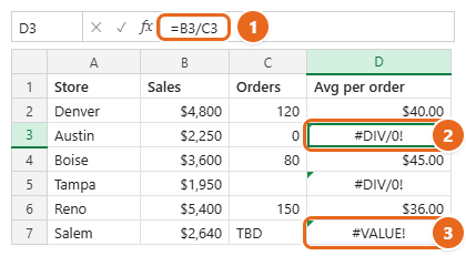
To replace those errors with a message:

1. Make sure the original formula is right. Check a row that should work, such as Denver. If the normal rows are wrong, fix that first. IFERROR only changes what you see when there’s an error.
2. Select the first formula cell. Click D2.
3. Wrap the formula. Type =IFERROR(B2/C2,"No orders") and press Enter. If you are editing an existing formula, click in the formula bar, type IFERROR( right after the equal sign, then type ,"No orders") at the end. As you type, Excel shows a tip with IFERROR(value, value_if_error) to remind you of the order.
4. Copy it down. Select D2, then drag the fill handle (the small square at the cell’s bottom-right corner) down to D7, or double-click the fill handle. The cell references update for each row.
5. Check the result. Denver, Boise and Reno still show their averages. Austin, Tampa and Salem now show No orders.

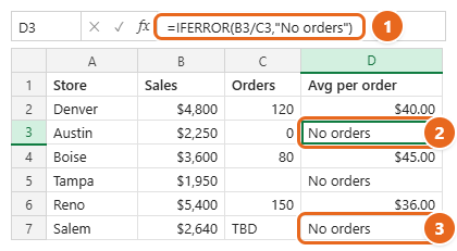
Look closely at Salem. Its order count isn’t zero, it’s a typo-style placeholder. IFERROR can’t tell the difference between “no orders yet” and “bad data”, so it shows the same message for both. Keep this in mind; the section When not to use IFERROR shows a more precise formula.

One formula for the whole column

In Excel for Microsoft 365, Excel 2024 and Excel 2021, you can give IFERROR whole ranges and let the results spill down. Clear D2:D7, click D2, and enter:

=IFERROR(B2:B7/C2:C7,"No orders")

Excel fills D2:D7 from that single formula. The cells below D2 must be empty, or you’ll see #SPILL!. In Excel 2019 and earlier, use the one-cell version and copy it down instead.

Use the Formulas tab instead of typing

If you’d rather not worry about commas and parentheses, let Excel build the formula. These steps are for Excel for Windows.

1. Click the cell where you want the result, such as D2.
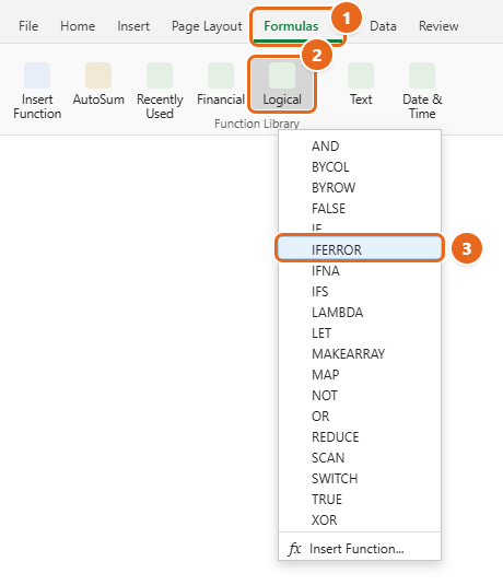
2. Select the Formulas tab, then select Logical in the Function Library group.
3. Choose IFERROR from the list.
   

   

4. In the Function Arguments box, type B2/C2 in Value.
5. Type "No orders" in Value_if_error. Include the quotation marks for text.
6. Select OK. The finished formula appears in the formula bar, and you can copy it down like any other formula.

You can also select Insert Function (the fx button next to the formula bar), search for IFERROR, and select Go to reach the same box. New to formulas in general? Using a formula in Excel covers the basics.

Choose what to show instead of the error

The second argument decides what readers see. Pick it based on what happens to the cell next.

Formula	Shows on error	Good for	Watch out for
=IFERROR(B2/C2,"No orders")	The text No orders	Reports people read	Text can’t be used in math later
=IFERROR(B2/C2,"")	A cell that looks blank	Clean dashboards and templates	The cell isn’t truly empty (see below)
=IFERROR(B2/C2,0)	0	Columns you add up	Zeros pull averages down
=IFERROR(B2/C2,D$10)	Whatever is in D10	One message you can change in one place	Lock the row with $ before copying down

What a “blank” from IFERROR really is

Two double quotes with nothing between them return empty text, not an empty cell. That matters in a few places:

• ISBLANK returns FALSE for the cell, because it contains a formula.
• COUNTA counts the cell as filled.
• COUNTBLANK does count it. The COUNTBLANK reference confirms that cells with formulas that return “” are counted as blank. Some guides say the opposite, so don’t rely on them for this.
• Math on the cell, such as =D3+5, returns #VALUE! because Excel can’t add a number to text. SUM and AVERAGE skip text in a range, so =SUM(D2:D7) still works.

If other formulas will do math on the result, use 0 or fix the cause instead of returning “”.

Use IFERROR with VLOOKUP and XLOOKUP

Lookups are the most common place to use IFERROR. When a lookup can’t find what you asked for, it returns #N/A. Say you have a price list in A2:B5 (Notebook, Pen, Stapler, Tape) and you look up items typed in column D. Marker isn’t in the list, so a plain VLOOKUP shows #N/A.

1. Click the result cell, E3 in this example.
2. Enter =IFERROR(VLOOKUP(D3,$A$2:$B$5,2,FALSE),"Not in list").
3. Press Enter, then copy the formula down. Items in the list show their price, and missing items show Not in list.

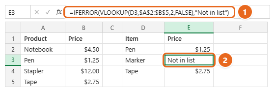
The dollar signs keep the price list range fixed while you copy the formula. If the lookup part is new to you, start with doing a VLOOKUP in Excel.

Better options for lookups: IFNA and XLOOKUP

For a lookup, the error you expect is #N/A. Other errors, such as #REF! after someone deletes a column, mean the formula is broken and you’d want to see them. Two options catch only the “not found” case:

• IFNA works like IFERROR but reacts only to #N/A: =IFNA(VLOOKUP(D3,$A$2:$B$5,2,FALSE),"Not in list"). It’s available in Excel 2013 and later, and the IFNA function reference has more examples.
• XLOOKUP has its own if_not_found argument, so it doesn’t need a wrapper: =XLOOKUP(D3,$A$2:$A$5,$B$2:$B$5,"Not in list"). XLOOKUP isn’t available in Excel 2016 or Excel 2019. The rest of its arguments are explained in doing an XLOOKUP in Excel.

Check a second list when the first one fails

Because value_if_error can be another formula, you can chain lookups. If discontinued products are on a sheet named Discontinued, this checks the main list first, then the second list, then gives up:

=IFERROR(VLOOKUP(D3,$A$2:$B$5,2,FALSE),IFERROR(VLOOKUP(D3,Discontinued!$A$2:$B$20,2,FALSE),"Not in list"))

Excel stops at the first lookup that works. Two or three levels are easy to follow. Beyond that, combining the lists into one table is usually simpler to maintain.

Add up or average a column that contains errors

A single error in a range breaks SUM. If column D still has the plain =B2/C2 formulas, =SUM(D2:D7) returns an error instead of a total. You have three ways around it:

• SUM with IFERROR: =SUM(IFERROR(D2:D7,0)) turns each error into 0 and adds the rest. In the sample, the result is 121 (40 + 45 + 36). In Excel for Microsoft 365, Excel 2024 and Excel 2021, just press Enter. In Excel 2019 and earlier, press Ctrl+Shift+Enter so it works as an array formula; Excel adds curly braces around it.
• AGGREGATE: =AGGREGATE(9,6,D2:D7) also returns 121. The 9 means SUM and the 6 means ignore error values. It needs no special keys in any current version.
• Wrap the source formulas: if column D uses =IFERROR(B2/C2,0) instead of =B2/C2, a plain =SUM(D2:D7) works.

Be careful with averages. Replacing errors with 0 counts those rows as real zeros. =AVERAGE(IFERROR(D2:D7,0)) returns about 20.17 (121 divided by 6), which is wrong for the three stores that had real results. To average only the valid numbers, use =AGGREGATE(1,6,D2:D7), where 1 means AVERAGE. It returns about 40.33 (121 divided by 3). Other ways to average are in calculating an average in Excel.

When not to use IFERROR

IFERROR hides every error, including ones that point to real mistakes. A misspelled function name (#NAME?), a deleted column (#REF!) and text in a number column (#VALUE!) all get the same friendly message. Use these habits to avoid hiding problems:

• Add IFERROR last. Build the formula, confirm it gives the right answers, then wrap it.
• Test for the expected problem instead. For the store report, =IF(C2=0,"No orders",B2/C2) handles zero and empty order counts (Excel treats an empty cell as 0 in this test). Salem’s TBD still shows #VALUE!, so you notice the bad entry and fix it. IF can handle more cases with multiple IF statements.
• Wrap the smallest part that can fail. In =IFERROR(VLOOKUP(D3,$A$2:$B$5,2,FALSE),0)*F3, only the lookup is protected. If the quantity in F3 is typed as text, you still see #VALUE! instead of a misleading 0.
• Use IFNA for lookups, as explained above.

Find errors before you hide them

To see every error on a sheet at once, select Home > Find & Select > Go To Special, choose Formulas, leave only Errors checked, and select OK. Excel selects each formula cell that currently shows an error, so you can review them before adding IFERROR.

The older IF and ISERROR method

You may see =IF(ISERROR(B2/C2),"No orders",B2/C2) in older workbooks. It gives the same result as IFERROR, but the formula has to be written twice. In any version from Excel 2007 on, IFERROR is shorter and easier to read. There’s no need to rewrite old formulas that work, though.

Troubleshooting

Excel reports a problem with this formula

Check the punctuation. Text must be in straight double quotes ("No orders", not curly quotes copied from a web page or document), there must be a comma between the two arguments, and every opening parenthesis needs a closing one. If your region uses a semicolon as the list separator, use ; instead of commas.

The formula itself shows #NAME?

IFERROR can catch a misspelled function inside it, but not a misspelling of IFERROR itself. Check that the formula starts with =IFERROR(, for example not =IFEROR(. Choosing the function from Formulas > Logical avoids typos.

You still see #SPILL!

When a spilled IFERROR formula is blocked by data in the cells below, the formula can’t place its results, so IFERROR has nothing to replace. Clear the cells in the spill range, or use the one-cell version and copy it down.

The cell shows the formula as text

The cell was probably formatted as Text before you typed the formula. Select the cell, select Home, set the number format box to General, then click in the formula bar and press Enter.

A lookup shows 0 instead of your message

That isn’t an error. VLOOKUP found the item, but the matching price cell is empty, so it returns 0. IFERROR only reacts to errors. Fill in the missing value, or hide zeros with a number format.

Every row shows the fallback value

The wrapped formula is failing everywhere, so something in the formula is wrong, such as a misspelled function name, a bad range or the wrong column number in VLOOKUP. Temporarily remove IFERROR to see the real error, fix it, then put IFERROR back.

FAQ

What is the difference between IFERROR and IFNA?

IFERROR reacts to every error type. IFNA reacts only to #N/A, which is the “not found” error from lookups. Use IFNA for lookups so that other errors stay visible.

Can IFERROR return a blank cell?

Yes. Use "" as the second argument, as in =IFERROR(B2/C2,""). The cell looks empty but contains empty text, so math such as =D3+5 on that cell returns #VALUE!.

Can I use IFERROR in Excel for Mac or Excel for the web?

Yes. IFERROR works in Excel for Microsoft 365 on Windows and Mac, Excel 2024 and 2021 for Windows and Mac, Excel 2019, Excel 2016 and Excel for the web. Typing the formula works the same way in each.

Can I nest IFERROR?

Yes. Put a second IFERROR in the value_if_error argument to try another formula when the first fails, as shown in the lookup section.

Does IFERROR fix the error?

No. It only changes what the cell displays. The underlying cause, such as a zero, a missing lookup value or bad data, is still there.

How do I remove IFERROR from a formula?

Click the cell, then in the formula bar delete IFERROR( after the equal sign and delete the comma, fallback value and last closing parenthesis at the end. Press Enter, then copy the corrected formula down if needed.

Next step

Pick one column in your workbook that shows errors, confirm the normal rows are correct, then wrap the formula with IFERROR and a clear message. If the column is a lookup, use IFNA or XLOOKUP’s built-in “not found” value instead, so real mistakes still show up.