How to Use COUNTIF in Excel

To use COUNTIF in Excel, click an empty cell and type =COUNTIF(range,criteria), then press Enter. For example, =COUNTIF(D2:D11,"Paid") counts how many cells in D2:D11 say Paid. The range is the cells to check, and the criteria is the condition a cell must meet, such as a word, a number, ">100" or a cell reference.

Applies to: Excel for Microsoft 365 (Windows, Mac and the web), Excel 2024, Excel 2021, Excel 2019 and Excel 2016. The one-formula summary that uses UNIQUE needs Microsoft 365, Excel 2024 or Excel 2021. Checked against Microsoft Support on October 12, 2026.

In this guide

• How COUNTIF works
• How to write a COUNTIF formula
• Build it with Insert Function instead
• COUNTIF criteria cheat sheet
• Count several values with one formula you copy down
• Count dates
• Count values between two numbers or dates
• Count this or that (OR logic)
• Find duplicates with COUNTIF
• COUNTIF, COUNTIFS, COUNT, COUNTA or COUNTBLANK?
• Troubleshooting
• FAQ

How COUNTIF works

COUNTIF looks through a group of cells and counts the ones that meet a single condition. It returns a number, and that number updates automatically when the data changes.

The syntax is:

=COUNTIF(range, criteria)

Argument	What to put there	Examples
range (required)	The cells you want Excel to check. This can be a column, a row, a block of cells or a named range.	D2:D11, A:A, Sales
criteria (required)	The condition a cell must meet to be counted: a number, text, a comparison or a cell reference.	"Paid", 100, ">100", H2

A few rules apply to every COUNTIF formula:

• Text and comparisons go in double quotation marks. Write "Paid" and ">100", not Paid or >100. A plain number such as 100 and a cell reference such as H2 don’t need quotes.
• It isn’t case-sensitive. paid, Paid and PAID all match "Paid".
• It checks one condition only. For two or more conditions, such as orders that are both Paid and in the East region, use COUNTIFS, covered later in this guide.
• It counts cells, not words. A cell that says Paid in full doesn’t match "Paid" unless you use a wildcard, explained in the criteria cheat sheet.

How to write a COUNTIF formula

The examples in this guide use a small order list in A1:F11 with the headers Order ID, Customer, Region, Status, Amount and Order Date. It has 10 orders: five are Paid, three are Pending and two are Overdue. Type a similar list into a blank sheet if you want to follow along.

1. Click the cell where you want the answer. Pick an empty cell outside your data, such as H2. Putting the result inside the range you’re counting can cause a circular reference warning.
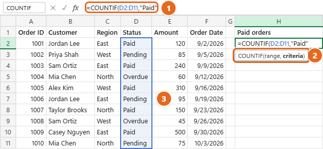
2. Start the formula. Type =COUNTIF(. Excel shows a small tip under the cell that reads COUNTIF(range, criteria), with the part you’re filling in shown in bold.
3. Enter the range. Drag across the cells you want to check, for example D2:D11, or type the address yourself. Excel outlines the selected cells in color so you can confirm the range. Don’t include the header row unless you want the header counted too.
4. Type a comma, then the condition. For the sample list, type "Paid" with the quotation marks. Type straight quotes from your keyboard. Curly quotes copied from a web page or a Word document make Excel reject the formula.
   

   

5. Close the formula and press Enter. Type ) and press Enter. The cell shows the count, which is 5 for the sample list. Click the cell again to see the full formula in the formula bar.
6. Check the result. If the number looks wrong, select the range and look at Count in the status bar at the bottom of the window, or filter the column for the value. The Troubleshooting section covers the usual reasons a count is off.

Tip: To check a whole column that keeps growing, use a full-column range such as =COUNTIF(D:D,"Paid"). Just make sure the formula itself isn’t in column D, and remember that the header in D1 is checked too.

Build it with Insert Function instead

If you’d rather fill in boxes than type the syntax, Excel for Windows can build the formula for you.

1. Click the cell where you want the result.
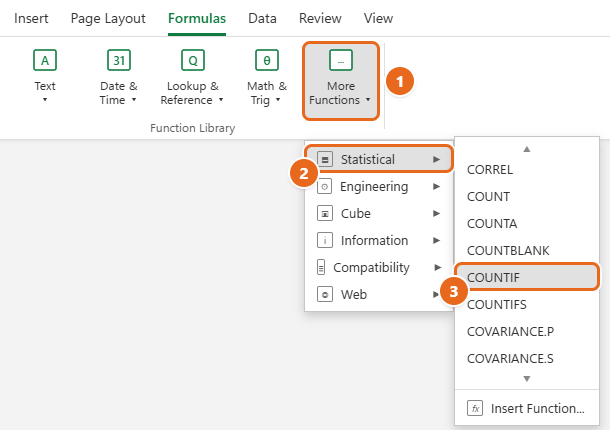
2. Select the Formulas tab. In the Function Library group, select More Functions > Statistical > COUNTIF. The list is in alphabetical order, so COUNTIF sits between COUNTBLANK and COUNTIFS.
   

   

3. In the Function Arguments dialog box, click in the Range box and select the cells to check on the sheet.
4. Click in the Criteria box and type your condition, such as "Paid" or ">100". Excel shows a preview of the answer next to Formula result near the bottom of the dialog box.
5. Select OK. Excel places the finished formula in the cell.

You can also select Insert Function (the fx button next to the formula bar), type countif in the search box, and select Go. In Excel for Mac, Insert Function opens a Formula Builder pane on the side of the window rather than a dialog box, but it asks for the same two arguments.

COUNTIF criteria cheat sheet

Almost everything you can do with COUNTIF comes down to what you put in the criteria. Each example below uses the sample order list, so you can compare your result with the answer shown.

To count cells that…	Formula	Result
Exactly match a word	=COUNTIF(D2:D11,"Paid")	5
Match the value in another cell	=COUNTIF(D2:D11,H2)	Depends on H2
Don’t match a word	=COUNTIF(D2:D11,"<>Paid")	5
Equal a number	=COUNTIF(E2:E11,150)	1
Are greater than a number	=COUNTIF(E2:E11,">100")	5
Are less than or equal to a number	=COUNTIF(E2:E11,"<=85")	4
Are greater than a number stored in a cell	=COUNTIF(E2:E11,">"&H5)	Depends on H5
Contain a word anywhere	=COUNTIF(B2:B11,"*Lee*")	2
Start with certain letters	=COUNTIF(B2:B11,"Sam*")	2
Have an exact length (one ? per character)	=COUNTIF(C2:C11,"????")	7
Contain any text	=COUNTIF(A1:F11,"*")	Text cells only
Are blank	=COUNTIF(D2:D11,"")	0
Aren’t blank	=COUNTIF(D2:D11,"<>")	10
Hold TRUE (for example, checked checkboxes)	=COUNTIF(G2:G11,TRUE)	Number of TRUE cells

What the symbols mean:

• Comparison operators: = equal to, > greater than, < less than, >= greater than or equal to, <= less than or equal to, and <> not equal to. The operator goes inside the quotes together with the value, as in ">=100".
• The ampersand (&): joins an operator to a cell or a function. ">"&H5 means “greater than whatever is in H5.” If you write ">H5" instead, Excel looks for the literal text >H5 and returns 0.
• Asterisk (*): stands for any number of characters, including none. "*Lee*" matches Jordan Lee and Lee Park.
• Question mark (?): stands for exactly one character. "????" matches the four-letter regions East and West but not North.
• Tilde (~): lets you count a real asterisk or question mark. "*~?*" counts cells that contain a question mark.

Note: Wildcards only work on text. A number such as 1050 isn’t matched by "*50", because Excel stores it as a number rather than as the characters 1, 0, 5 and 0. Use a comparison such as ">=1000" for numbers instead.

Count several values with one formula you copy down

Rather than writing a separate formula for each status, put the values you want to count in cells and point one formula at them. This is easier to update and less likely to contain typos.

1. In H1, type Status, and in I1, type Orders.
2. In H2, H3 and H4, type Paid, Pending and Overdue.
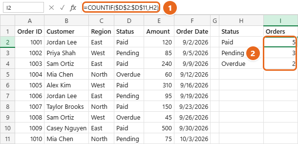
3. Click I2 and type =COUNTIF($D$2:$D$11,H2), then press Enter. The dollar signs lock the range so it doesn’t move when you copy the formula. H2 has no dollar signs, so it moves down one row at a time.
4. Select I2, then drag the small square at the bottom-right corner of the cell (the fill handle) down to I4. Excel fills in the counts for each status.
   

   

5. Check the total. The counts in I2:I4 should add up to the number of orders, which is 10 in the sample. If they don’t, some cells probably contain a different spelling or extra spaces.

Forgetting the dollar signs is the most common mistake here. Without them, the range shifts to D3:D12, then D4:D13, and the counts quietly go wrong. Our guide on how to keep one cell constant in Excel explains absolute references in more detail. You can press F4 on Windows while the cursor is in a cell reference to add the dollar signs.

Count every value automatically (Microsoft 365, Excel 2024 and 2021)

If you don’t know all the values ahead of time, let Excel list them for you:

1. In K2, type =UNIQUE(D2:D11). Excel spills each different status into K2 and the cells below it.
2. In L2, type =COUNTIF(D2:D11,K2#). The # after K2 refers to the whole spilled list, so this single formula returns one count for each status.

When a new status appears in the data, both lists grow on their own. If you see a #SPILL! error, something is in the way. Clear the cells below the formula and it will fill them. For other ways to tally values, including PivotTables, see how to count the number of occurrences in Excel.

Count dates

Excel stores dates as serial numbers, so you count them with the same comparison operators you use for numbers. The sample list has order dates in F2:F11, from September 2 to October 3, 2026.

To count…	Formula
Orders on one date	=COUNTIF(F2:F11,DATE(2026,9,16))
Orders on or after a date	=COUNTIF(F2:F11,">="&DATE(2026,9,15))
Orders before a date in a cell	=COUNTIF(F2:F11,"<"&H8)
Orders dated today	=COUNTIF(F2:F11,TODAY())
Orders in the past (before today)	=COUNTIF(F2:F11,"<"&TODAY())
Orders in the next 7 days	=COUNTIFS(F2:F11,">="&TODAY(),F2:F11,"<="&TODAY()+7)

You can type a date straight into the criteria, such as ">=9/15/2026", and it works in US English Excel. The DATE function is safer when you share the workbook, because DATE(2026,9,15) means September 15, 2026 no matter which date format the other person’s computer uses.

If a date count comes back 0, check that the dates are real dates. Dates imported as text are usually left-aligned in the cell and won’t match a comparison.

Count values between two numbers or dates

COUNTIF only takes one condition, so “between” needs either COUNTIFS or two COUNTIFs subtracted from each other. To count orders from $100 to $300, including both ends:

• With COUNTIFS (easiest to read): =COUNTIFS(E2:E11,">=100",E2:E11,"<=300")
• With two COUNTIFs: =COUNTIF(E2:E11,">=100")-COUNTIF(E2:E11,">300")

Both return 3 for the sample list (120, 240 and 150). The subtraction version counts everything at or above the lower limit, then takes away everything above the upper limit.

Watch the operators. Subtracting COUNTIF(E2:E11,"<=300") instead of COUNTIF(E2:E11,">300") doesn’t give you a “between” count. It gives you the number of values above 300. And if you want to leave out the end points, change the operators: ">100" and "<300" in COUNTIFS. Decide whether the limits themselves should count before you write the formula.

The same pattern works for dates. =COUNTIFS(F2:F11,">="&DATE(2026,9,1),F2:F11,"<="&DATE(2026,9,30)) counts the September orders, which is 9 in the sample.

Count this or that (OR logic)

To count cells that match one value or another in the same column, add two COUNTIFs together:

=COUNTIF(D2:D11,"Paid")+COUNTIF(D2:D11,"Pending")

This returns 8. For a longer list of values, put them in braces, an array constant, and wrap the formula in SUM:

=SUM(COUNTIF(D2:D11,{"Paid","Pending","Overdue"}))

Adding COUNTIFs works safely in a single column because one cell can’t be Paid and Pending at the same time. Be careful when the conditions overlap or are in different columns. For example, =COUNTIF(C2:C11,"East")+COUNTIF(D2:D11,"Paid") counts an order that is both East and Paid twice. To count those rows once, subtract the overlap: =COUNTIF(C2:C11,"East")+COUNTIF(D2:D11,"Paid")-COUNTIFS(C2:C11,"East",D2:D11,"Paid"), which returns 6 for the sample.

Find duplicates with COUNTIF

Because COUNTIF can count how often a value appears, it’s a quick way to spot repeats before you delete anything.

1. Add a helper column next to your data, for example G, and type Repeat? in G1.
2. In G2, type =COUNTIF($B$2:$B$11,B2)>1 and press Enter.
3. Copy the formula down to G11. Each customer who appears more than once shows TRUE. In the sample, Jordan Lee, Sam Ortiz and Mia Chen each show TRUE twice.

To flag only the second and later copies, so the first one is kept, use an expanding range instead: =COUNTIF($B$2:B2,B2)>1. Only the first part of the range is locked, so the range grows as you copy the formula down.

You can also use COUNTIF as a conditional formatting rule. Select B2:B11, select Home > Conditional Formatting > New Rule > Use a formula to determine which cells to format, enter =COUNTIF($B$2:$B$11,B2)>1, select Format to pick a fill color, and select OK twice. For more rule ideas, see how to color cells in Excel based on value.

COUNTIF, COUNTIFS, COUNT, COUNTA or COUNTBLANK?

Excel has several counting functions, and picking the right one saves you from forcing COUNTIF to do something it isn’t built for.

Function	What it counts	Example
COUNTIF	Cells that meet one condition	=COUNTIF(D2:D11,"Paid")
COUNTIFS	Rows that meet every condition you list (AND logic)	=COUNTIFS(C2:C11,"East",D2:D11,"Paid") returns 3
COUNT	Cells that contain numbers, including dates	=COUNT(E2:E11)
COUNTA	Cells that aren’t empty	=COUNTA(B2:B11)
COUNTBLANK	Empty cells	=COUNTBLANK(D2:D11)

COUNTIFS uses pairs of range and criteria: =COUNTIFS(range1,criteria1,range2,criteria2,...). According to Microsoft, you can use up to 127 pairs, and every range must have the same number of rows and columns, though the ranges don’t have to sit next to each other. See Microsoft’s COUNTIFS function page for more examples.

If you need to add up amounts rather than count rows, such as the total of all paid orders, use SUMIF instead: =SUMIF(D2:D11,"Paid",E2:E11). Our SUMIF guide walks through it. For the other counting functions, see how to count the number of cells in Excel.

Case-sensitive counts

COUNTIF can’t tell paid from Paid. When capitalization matters, such as with product codes, use SUMPRODUCT with EXACT: =SUMPRODUCT(--EXACT(D2:D11,"Paid")). EXACT compares each cell with the text, including capital letters, and the two minus signs turn TRUE and FALSE into 1 and 0 so SUMPRODUCT can add them.

Troubleshooting

COUNTIF returns 0, but the value is clearly there

• Extra spaces or hidden characters. Paid with a trailing space doesn’t match "Paid". Microsoft also lists curly quotation marks and nonprinting characters as causes. Clean the data with TRIM or CLEAN in a helper column, or count with wildcards as a quick check: if "*Paid*" finds more cells than "Paid", some cells contain extra characters.
• A missing ampersand. ">H5" looks for the text >H5. Write ">"&H5.
• Text instead of numbers or dates. Numbers and dates imported from other systems are sometimes stored as text, often with a small green triangle in the corner of the cell. Comparisons such as ">100" skip them. Select the cells, select the warning icon, and choose Convert to Number if it’s offered.
• The wrong range. Click the formula and check the colored outline on the sheet. Make sure it covers every row of data.

Excel says there’s a problem with the formula

Look for curly quotation marks copied from a website or a document, a missing comma between the range and the criteria, or a missing closing parenthesis. Retype the quotation marks from your keyboard. In some regions, Excel uses a semicolon instead of a comma between arguments, as in =COUNTIF(D2:D11;"Paid").

The formula shows as text instead of a result

The cell was formatted as Text before you typed the formula. Select the cell, select Home and change the number format to General, then click in the formula bar and press Enter to re-enter the formula. Also make sure the formula starts with an equal sign and has no space before it.

The count is wrong after copying the formula down

The range moved with the formula. Add dollar signs to lock it, as in $D$2:$D$11, then copy the formula again.

#VALUE! when counting from another workbook

Microsoft notes that COUNTIF returns #VALUE! when it refers to a range in another workbook that is closed. Open the other workbook, and the formula recalculates. If you need the formula to work while the other file is closed, copy the data into the current workbook.

Wrong results with very long text

COUNTIF gives incorrect results when it matches strings longer than 255 characters. Microsoft’s workaround is to split the long text and join it with the & operator in the criteria, such as "first part"&"second part".

Excel won’t accept the range

The range argument has to be cells on a worksheet. If you try to give COUNTIF the result of another function as its range, such as a filtered list built with FILTER, Excel won’t accept the formula. Point COUNTIF at the original cells, or use COUNTIFS to add the extra condition. The criteria argument is more flexible and can take a spilled range like K2#.

FAQ

Can COUNTIF count cells by color?

No. COUNTIF only looks at values, not fill or font color. Microsoft suggests a custom VBA function for counting by color. A simpler approach is to count by the same rule that colored the cells, for example =COUNTIF(D2:D11,"Overdue") if overdue orders are shaded red. If you colored cells by hand, you can filter the column by color and read the count in the status bar.

Can I use COUNTIF with two criteria?

Not in one COUNTIF. For rows that must meet both conditions, use COUNTIFS. For cells that can meet either condition, add two COUNTIFs together, as shown in the OR logic section.

How do I count cells that contain specific text?

Put an asterisk on both sides of the text: =COUNTIF(B2:B11,"*Lee*"). To use a word stored in a cell, join the asterisks with ampersands: =COUNTIF(B2:B11,"*"&H2&"*").

Does COUNTIF count blank cells?

Only if you ask it to. =COUNTIF(D2:D11,"") counts empty cells, and =COUNTIF(D2:D11,"<>") counts cells that aren’t empty. COUNTBLANK and COUNTA do the same jobs and are easier to read.

Can I count across several sheets?

COUNTIF’s range must be on one sheet, so add one COUNTIF per sheet: =COUNTIF(Jan!D2:D50,"Paid")+COUNTIF(Feb!D2:D50,"Paid"). If you add more sheets often, consider stacking the data on one sheet first.

Does COUNTIF work in Excel for the web, Mac and Google Sheets?

Yes. COUNTIF works the same way in Excel for Windows, Excel for Mac and Excel for the web, and the formulas in this guide can be typed directly into any of them. Google Sheets also has a COUNTIF function with the same two arguments.

What is the difference between COUNTIF and SUMIF?

COUNTIF tells you how many cells meet a condition. SUMIF adds up the numbers in the rows that meet it. With the sample list, =COUNTIF(D2:D11,"Paid") returns 5 orders, and =SUMIF(D2:D11,"Paid",E2:E11) returns $1,320, the total value of those orders.

Once you’re comfortable with COUNTIF, try turning one of your own lists into a small summary table with criteria in cells, as in the summary table section. It’s the quickest way to get a live count of anything you track in Excel.