How to Remove Duplicates in Excel

To remove duplicates in Excel, click any cell in your data, then select Data > Remove Duplicates. Check My data has headers if your first row holds column names, tick the columns that must match for two rows to count as duplicates, and select OK. Excel keeps the first copy of each row, deletes the rest, and tells you how many it removed.

Applies to: Excel for Microsoft 365 (Windows, Mac and the web), Excel 2024, Excel 2021, Excel 2019 and Excel 2016. The UNIQUE function needs Microsoft 365, Excel 2024 or Excel 2021. Checked against Microsoft Support on October 12, 2026.

In this guide

• Which method should you use?
• Before you start: how Excel decides what is a duplicate
• Method 1: Use the Remove Duplicates button
• Check first: highlight duplicates without deleting them
• Method 2: Copy a clean list with Advanced Filter
• Method 3: Use the UNIQUE function
• Method 4: Flag or remove every copy with COUNTIF
• Method 5: Remove duplicates with Power Query
• How to undo Remove Duplicates
• Troubleshooting
• FAQ

Which method should you use?

Every method below ends with a list where each record appears once. The real difference is whether your original data is changed.

Method	Changes your original data?	Best for
Remove Duplicates button	Yes, deletes rows in place	A quick, one-time cleanup
Conditional formatting	No, only colors cells	Seeing what would be removed before you delete anything
Advanced Filter	No, when you copy to another location	A clean copy next to the original, in any version
UNIQUE function	No	A list that updates itself when the source changes
COUNTIF helper column	Only when you delete flagged rows	Removing every copy, or reviewing duplicates one by one
Power Query	No, it loads a new table	The same messy import you clean every week or month

If you only need to clean a list once and you have a backup, use Method 1. If you are not sure the duplicates are real mistakes, highlight them first.

Before you start: how Excel decides what is a duplicate

The examples in this guide use a small sign-up list in A1:D13 with the headers Name, Email, City and Signed Up. Three people, such as Jordan Lee ([email protected], Denver), signed up twice on different dates.

• A duplicate is decided by the columns you choose. If you compare Name, Email and City, two rows are duplicates only when all three match. The Signed Up date is ignored, so Jordan Lee’s second sign-up is removed even though the date is different.
• The whole row goes, not just the cell. When your whole table is selected, Excel deletes the entire duplicate row within that range. Cells outside the selected range are not changed or moved.
• The first copy stays. Excel keeps the first row it finds, working from the top down. If you want to keep the newest entry instead, sort by date from newest to oldest before you remove duplicates.
• Excel compares what the cell displays. According to Microsoft, the same date shown as 12/8/2026 in one cell and Dec 8, 2026 in another is treated as two different values. Two cells with different formulas that show the same result, such as =2-1 and =3-2, count as duplicates.
• Capital letters don’t matter. Remove Duplicates treats JORDAN LEE and Jordan Lee as the same value. Power Query is the exception, as explained in Method 5.
• Extra spaces do matter. Jordan Lee with a trailing space is a different value from Jordan Lee without one. See Troubleshooting for a fix.

Important: Remove Duplicates permanently deletes data. Save a copy of the workbook, or copy the sheet (right-click the sheet tab > Move or Copy > check Create a copy), before you continue.

Method 1: Use the Remove Duplicates button

This works the same way in Excel for Windows, Excel for Mac and Excel for the web.

1. Remove outlines and subtotals. Remove Duplicates doesn’t work on data that is outlined or has subtotals. If you added subtotals, select Data > Subtotal > Remove All first.
2. Select your data. Click any cell inside the list. Excel selects the whole block of connected data for you. If your list has blank rows or blank columns in the middle, select the full range yourself instead, from the header row to the last row.
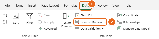
3. Open Remove Duplicates. Select the Data tab, then select Remove Duplicates in the Data Tools group. On Windows, you can also press Alt, then A, then M, one key at a time. In a narrow window, Data Tools may shrink to icons only; the Remove Duplicates icon shows two rows with a red X.
   

   

4. Answer the warning, if you see one. If you selected only one column and there is data in the columns next to it, a Remove Duplicates Warning appears. Choose Expand the selection to compare and delete whole rows, which keeps each row’s data together. Choose Continue with the current selection only if the column is a standalone list. Then select Remove Duplicates.
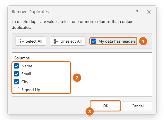
5. Check My data has headers. In the Remove Duplicates dialog box, leave My data has headers checked when row 1 holds column names, so the headers are never compared or deleted. When it is checked, the list shows your header names. When it is cleared, the list shows Column A, Column B and so on.
6. Choose the columns that must match. Under Columns, check each column that should be identical for two rows to count as duplicates. Use Select All to delete only rows that are exact copies, or Unselect All and then check just the columns you need. In the sample list, check Name, Email and City, and clear Signed Up.
   

   

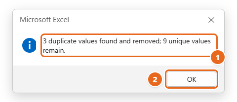
7. Select OK. Excel deletes the duplicate rows and shows a message such as 3 duplicate values found and removed; 9 unique values remain. Microsoft notes that these counts can include empty cells and spaces. Select OK to close the message.
   

   

8. Check the result. Scroll through the list, or select the column and look at Count in the status bar at the bottom of the window. If the number looks wrong, press Ctrl+Z right away.

Choosing columns: a quick example

Which boxes you tick changes the result a lot. Using the sample sign-up list:

• Email only: any repeated email address is removed, even if the name is spelled differently. This is often the most reliable choice for contact lists, because an email address identifies one person.
• Name, Email and City: a row is removed only when all three match. A second sign-up from the same person in the same city is removed.
• All four columns: nothing is removed in the sample, because every repeat sign-up has a different date.

Rule of thumb: fewer ticked columns remove more rows. Tick only the columns that truly identify a record, and leave out notes, timestamps and amounts that can differ between real duplicates.

Remove duplicates from an Excel table

If your data is formatted as a table, click anywhere in it, then select Table Design > Remove Duplicates in the Tools group. The same dialog box opens. The Data > Remove Duplicates button works for tables too. Not sure whether your data is a table? See how to create a table in Excel.

Check first: highlight duplicates without deleting them

Microsoft recommends reviewing duplicates before you remove them. Conditional formatting colors repeated values and deletes nothing.

1. Select the cells to check, for example the Email column.
2. Select Home > Conditional Formatting > Highlight Cells Rules > Duplicate Values.
3. In the Duplicate Values box, leave the first list set to Duplicate and pick a format next to values with. The default is Light Red Fill with Dark Red Text.
4. Select OK. Every copy of a repeated value is colored, including the first one.

To see only the highlighted rows, turn on Data > Filter, select the arrow in that column, and choose Filter by Color. To remove the highlighting later, select Home > Conditional Formatting > Clear Rules > Clear Rules from Selected Cells. Note that this rule can’t highlight duplicates in the Values area of a PivotTable. For more ways to color cells with rules, see how to color cells in Excel based on value.

Method 2: Copy a clean list with Advanced Filter

Advanced Filter can copy one instance of each row to a new spot and leave your original list untouched. It works in every desktop version of Excel. It compares every column in the range you give it, so a row is skipped only when the whole row matches another row.

1. Click any cell in your list.
2. Select Data > Advanced in the Sort & Filter group. The Advanced Filter dialog box opens.
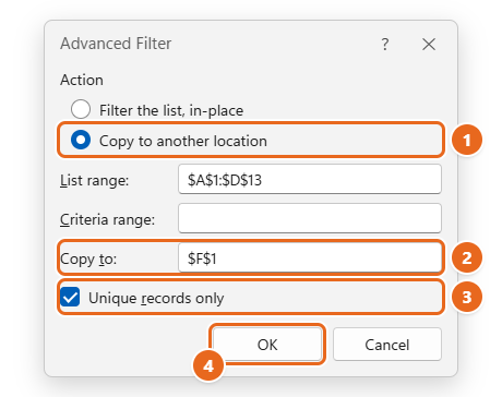
3. Under Action, select Copy to another location.
4. Check that List range covers your data, including the header row, such as $A$1:$D$13. Leave Criteria range empty.
5. Click in Copy to, then click an empty cell with enough empty space below and to the right, such as F1.
6. Check Unique records only, then select OK. The unique rows, with headers, appear starting at the cell you chose.
   

   

To compare only some columns, set the List range to just those columns. If you choose Filter the list, in-place instead, Excel hides the duplicate rows rather than deleting them. Select Data > Clear to show them again.

Tip: Excel copies filtered results to the sheet you are on. If you want the clean list on a different sheet, go to that sheet first, click an empty cell, open Advanced, and then select the List range on the original sheet.

Method 3: Use the UNIQUE function

In Excel for Microsoft 365, Excel 2024, Excel 2021 and Excel for the web, the UNIQUE function builds a duplicate-free list with one formula. Your original data stays as it is, and the result updates when the source changes.

1. Click an empty cell with plenty of empty space below it, such as F2.
2. Type =UNIQUE(B2:B13) and press Enter. Each email address appears once, and the list spills into the cells below.
3. To compare whole rows instead, include every column you want to compare, for example =UNIQUE(A2:C13) for Name, Email and City. A row is left out only when every column in the range matches.

The full syntax is =UNIQUE(array, [by_col], [exactly_once]):

• array is the range to check.
• by_col is optional. Leave it out, or use FALSE, to compare rows. Use TRUE to compare columns across a horizontal list.
• exactly_once is optional. Use TRUE to list only values that appear exactly once, for example =UNIQUE(B2:B13,,TRUE) returns people who signed up a single time.

Useful variations:

• Sorted list: =SORT(UNIQUE(B2:B13))
• Skip blank cells: =UNIQUE(FILTER(B2:B13,B2:B13<>""))
• Only one city: =UNIQUE(FILTER(A2:A13,C2:C13="Denver"))

If you see #SPILL!, something is in the way of the results. Clear the cells below the formula. To turn the result into plain values that no longer change, select the spilled list, copy it, then select Home > Paste > Paste Values in another spot. If your data is formatted as a table and the formula uses structured references, the result grows automatically as you add rows. Microsoft’s UNIQUE function reference has more examples.

Method 4: Flag or remove every copy with COUNTIF

Remove Duplicates always keeps one copy. If you want to delete both copies of a repeated record, or look at each duplicate before deciding, use a helper column. This works in every version of Excel.

1. In E1, type a header such as Repeat?.
2. In E2, enter one of these formulas, then drag the fill handle (the small square at the cell’s bottom-right corner) down to the last row:
   • =COUNTIF($B$2:$B$13,B2)>1 shows TRUE on every copy of a repeated email, including the first.
   • =COUNTIF($B$2:B2,B2)>1 shows TRUE only on the second and later copies, so the first copy is kept.
3. Select Data > Filter, open the arrow on the Repeat? column, and show only TRUE.
4. Select the visible row numbers, right-click, and choose Delete Row. Only the visible rows are deleted.
5. Turn off the filter and delete the helper column.

To match on more than one column, use COUNTIFS, for example =COUNTIFS($A$2:$A$13,A2,$B$2:$B$13,B2)>1. COUNTIF isn’t case-sensitive either. If capitals matter, for example in product codes, use =SUMPRODUCT(--EXACT($B$2:$B$13,B2))>1. To count how many times each value appears instead, see how to count the number of occurrences in Excel.

Method 5: Remove duplicates with Power Query

Power Query saves your cleanup steps, so next time you only need to refresh. It’s built into Excel for Microsoft 365 and Excel 2016 and later on Windows. Excel for Mac has more limited Power Query support, so these steps are written for Windows. If you can’t find it, see how to find and enable Power Query in Excel.

1. Click a cell in your data and select Data > From Table/Range in the Get & Transform Data group. If the data isn’t a table yet, confirm the range in the Create Table box and select OK. The Power Query Editor opens.
2. Select the column headers that define a duplicate. Hold Ctrl to select more than one, or press Ctrl+A to select all columns.
3. Select Home > Remove Rows > Remove Duplicates.
4. Select Home > Close & Load. The clean data loads into a new sheet as a table. Your original data isn’t changed.
5. When the source data changes, select Data > Refresh All to run the same steps again.

Two differences from the Remove Duplicates button matter, according to Microsoft Learn:

• Power Query is case-sensitive. Jordan Lee and JORDAN LEE are different. To ignore case, select the column and choose Transform > Format > lowercase (or UPPERCASE) before you remove duplicates.
• It doesn’t promise to keep the first copy. If it matters which copy survives, use the Remove Duplicates button on sorted data instead.

How to undo Remove Duplicates

• Right away: press Ctrl+Z (Command+Z on a Mac), or select Undo. All the deleted rows come back.
• After saving, if the file is on OneDrive or SharePoint: select File > Info > Version History and open an earlier version.
• Otherwise: open the backup copy you made before you started. Once a local file is saved and closed, the deleted rows can’t be recovered from Excel.

Troubleshooting

Remove Duplicates is grayed out

• You may still be typing in a cell. Press Enter or Esc first.
• The sheet may be protected. Select Review > Unprotect Sheet. If it asks for a password you don’t have, ask the file’s owner.

Excel says no duplicates were found, but you can see them

• Extra spaces or hidden characters. In a helper column, use =TRIM(CLEAN(B2)), copy it down, paste it back over the original as values, then try again.
• Numbers stored as text. A number with a small green triangle in the corner is stored as text and doesn’t match a real number. Select the cells, select the warning icon, and choose Convert to Number.
• Different formats. Dates or numbers shown in different formats count as different values. Apply the same number format to the whole column.
• Too many columns ticked. If a timestamp or notes column is ticked, rows that differ only there are not duplicates. Clear those columns in the dialog.

The wrong data was deleted or rows got mixed up

This usually happens when Continue with the current selection was chosen for one column inside a larger table. Values in that column shift and no longer line up with the rest of their row. Press Ctrl+Z and run it again with Expand the selection.

You get a message about outlines or subtotals

Remove the subtotals with Data > Subtotal > Remove All, and remove grouping with Data > Ungroup > Clear Outline. Then try again.

Empty rows disappeared

Blank rows inside your range are compared like any other row, so extra blank rows count as duplicates of the first one and are removed. If you need those blank rows, leave them out of the selection.

Stop new duplicates from being entered

To block repeats as people type, select the column (for example B2:B500), then select Data > Data Validation. Under Allow, choose Custom, enter =COUNTIF($B$2:$B$500,B2)=1 in Formula, and select OK. Excel now rejects any value that is already in the column. Data Validation doesn’t check values that are pasted in, so run Remove Duplicates now and then as well.

FAQ

Does Remove Duplicates keep the first or the last entry?

It keeps the first one, from the top of the range. To keep the most recent entry, sort the data by date from newest to oldest first.

Is there a keyboard shortcut for Remove Duplicates?

On Windows, press Alt, A, M in sequence. Excel for Mac doesn’t use this ribbon shortcut, so use the Data tab.

How do I remove duplicates based on one column but keep the other columns?

Select the whole data range, or click a cell in it, open Remove Duplicates, select Unselect All, and check only the column to match on. Excel removes the entire row each time that column repeats, so the other columns stay lined up.

Can I remove duplicates in Excel for the web or on a Mac?

Yes. Microsoft lists Data > Remove Duplicates for Excel for Microsoft 365, Excel for Mac and Excel for the web. The steps are the same as Method 1.

How do I remove both copies of a duplicate?

Use the COUNTIF helper column in Method 4 with =COUNTIF($B$2:$B$13,B2)>1, filter for TRUE, and delete the visible rows. To simply list the values that appear only once, use =UNIQUE(range,,TRUE).

Can I remove duplicates across two columns or two lists?

Remove Duplicates compares rows, so two side-by-side lists are not compared with each other. Paste one list under the other in a single column first, then remove duplicates from that column. With UNIQUE, you can combine lists in one formula: =UNIQUE(VSTACK(A2:A20,C2:C20)) in Microsoft 365 and Excel 2024.

Next step

Before you run Remove Duplicates on real data, save a copy and highlight the duplicates with conditional formatting to confirm what will go. Then use the Remove Duplicates button for a one-time cleanup, or set up UNIQUE or Power Query if the list keeps changing.