How to Do a VLOOKUP in Excel (With Examples)

VLOOKUP finds a value in the first column of a table and returns something from the same row, such as looking up a product ID to get its price. The formula is =VLOOKUP(what to find, where to look, which column to return, FALSE). The FALSE at the end asks for an exact match, and leaving it out is the most common reason VLOOKUP returns the wrong answer. This guide builds a VLOOKUP step by step, explains each part, and fixes the errors you’re most likely to see.

The example

Say you have a price list in columns E to G: product ID in E, product name in F, and price in G. In column A you have a list of product IDs from an order, and you want each one’s price in column B.

How to write a VLOOKUP, step by step

1. Click cell B2, where you want the first price to appear.
2. Type =VLOOKUP(
3. Lookup value: click A2, the ID you want to find, then type a comma.
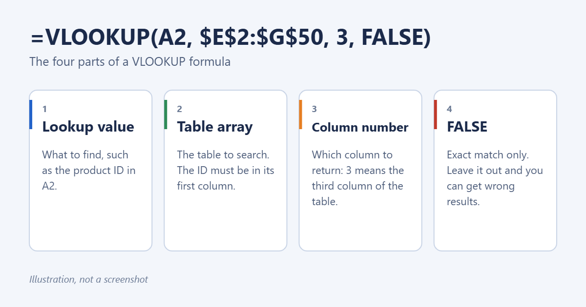
4. Table array: select the price list, E2:G50. Press F4 once to turn it into $E$2:$G$50 so it doesn’t shift when you copy the formula down. Type a comma.
5. Column index number: type 3, because price is the third column of the range E:G. Type a comma.
6. Range lookup: type FALSE for an exact match, then close the bracket and press Enter.

The finished formula is:

=VLOOKUP(A2,$E$2:$G$50,3,FALSE)

Double-click the small square at the bottom-right of B2 to copy the formula down the rest of the column. Each row looks up its own ID.

What each part means

• Lookup value is what you’re searching for. It can be a cell reference, a number, or text in quotes, like "SKU-104".
• Table array is the range to search. VLOOKUP only searches its first column, so the value you’re looking for has to be on the left.
• Column index number counts from the first column of the table array, not from column A. In E:G, E is 1, F is 2, and G is 3.
• Range lookup is FALSE (or 0) for an exact match, or TRUE for an approximate match. If you leave it out, Excel uses TRUE.

Exact match vs. approximate match

Use FALSE almost every time. With TRUE, VLOOKUP assumes the first column is sorted smallest to largest and returns the closest value that isn’t larger than the one you’re looking for. That’s useful for tax brackets, grading scales, or shipping rates by weight, but on an unsorted list it quietly returns the wrong row.

Example of a valid approximate match: with score thresholds 0, 60, 70, 80, 90 sorted in column E and grades F, D, C, B, A in column F, =VLOOKUP(A2,$E$2:$F$6,2,TRUE) turns a score of 84 into a B.

VLOOKUP from another sheet

The price list doesn’t have to be on the same sheet. While writing the formula, click the other sheet’s tab and select the range there. Excel writes the sheet name for you:

=VLOOKUP(A2,Prices!$A$2:$C$50,3,FALSE)

See how to do a VLOOKUP between two sheets for more, including looking up from a different workbook.

Fixing common VLOOKUP errors

#N/A

Excel couldn’t find the lookup value. Check for:

• Extra spaces. “SKU-104 ” with a trailing space doesn’t match “SKU-104”. Clean the data with =TRIM(A2).
• Numbers stored as text. A green triangle in the corner of a cell is a clue. Select the cells, click the warning icon, and choose Convert to Number.
• The value isn’t in the first column. VLOOKUP can’t look to the left. Move the column, or use XLOOKUP instead.
• The value really isn’t there. To show a friendly message instead of #N/A, wrap the formula: =IFERROR(VLOOKUP(A2,$E$2:$G$50,3,FALSE),"Not found").

#REF!

The column index number is larger than the number of columns in the table array. If the range is E:G, the highest you can use is 3.

Wrong results

Usually the last argument is missing or set to TRUE on unsorted data. Add FALSE. If the results are right in the first row but wrong further down, the table range wasn’t locked with dollar signs. See how to keep one cell constant in Excel for more on dollar signs.

Results break after inserting a column

The column index number is fixed, so inserting a column inside the table shifts the data but not the number. Update the number, or switch to XLOOKUP, which doesn’t use one.

Return more than one column

To pull the name and the price at once, change the column index for each copy of the formula, or in Microsoft 365 use an array: =VLOOKUP(A2,$E$2:$G$50,{2,3},FALSE) spills both values into two cells. Our guide on using VLOOKUP for multiple columns covers other options.

Should you use XLOOKUP instead?

If you have Microsoft 365 or Excel 2021 or later, XLOOKUP is easier: =XLOOKUP(A2,$E$2:$E$50,$G$2:$G$50,"Not found"). It looks in any direction, defaults to an exact match, and doesn’t break when you insert columns. VLOOKUP is still worth knowing because it works in every version of Excel and in files other people send you. See how to do an XLOOKUP in Excel.

Frequently asked questions

Is VLOOKUP case-sensitive?

No. “abc” and “ABC” are treated as the same value.

What if there are duplicates in the lookup column?

VLOOKUP returns the first match it finds, starting from the top.

Can VLOOKUP use wildcards?

Yes, with an exact match. =VLOOKUP("*smith*",$E$2:$G$50,2,FALSE) finds the first entry containing “smith.”

Summary

Use =VLOOKUP(lookup value, table, column number, FALSE), make sure the value you’re finding is in the table’s first column, and lock the table with dollar signs before copying the formula down.

Related: How to Match Data in Excel from 2 Worksheets.