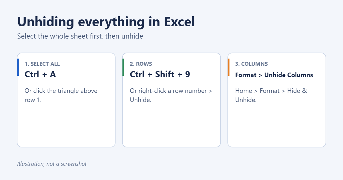
To unhide all rows in Excel, select the whole sheet by pressing Ctrl + A (or clicking the small triangle above row 1), then right-click any row number and choose Unhide. The keyboard shortcut is Ctrl + Shift + 9. To unhide every column too, keep the sheet selected and go to Home > Format > Hide & Unhide > Unhide Columns. If rows still won’t appear, they’re probably filtered, grouped, or set to zero height rather than hidden. Fixes for each case are below.
Unhide all rows
- Click the Select All triangle where the row numbers and column letters meet, or press Ctrl + A (twice if you’re inside a table).
- Right-click any row number and choose Unhide.
Or, with the sheet selected, go to Home > Format > Hide & Unhide > Unhide Rows, or press Ctrl + Shift + 9.
Unhide all columns
- Select the whole sheet as above.
- Right-click any column letter and choose Unhide, or go to Home > Format > Hide & Unhide > Unhide Columns.
The shortcut Ctrl + Shift + 0 is meant to unhide columns, but Windows often reserves it for switching keyboard languages, so it may do nothing. Use the menu instead.
Unhide specific rows or columns
To reveal only rows 5 to 9, for example, select rows 4 and 10 (the visible rows on either side), right-click, and choose Unhide. The same works for columns.
Unhide row 1 or column A
You can’t select the row above row 1. Instead, type A1 in the Name Box to the left of the formula bar and press Enter, then use Home > Format > Hide & Unhide > Unhide Rows (or Unhide Columns for column A).
Rows still missing? Check these
A filter is on
If row numbers turn blue and some are skipped, a filter is hiding rows. Go to Data > Clear to show all rows, or click Filter to turn filtering off.
The rows are grouped
Small + buttons in the margin to the left of the row numbers mean the rows are grouped and collapsed. Click the + buttons, or the highest number at the top of the margin, to expand them all. To remove the grouping, select the rows and choose Data > Ungroup.
The row height is very small
A row set to a tiny height looks hidden but isn’t. Select the sheet, go to Home > Format > Row Height, enter 15, and click OK. Or use AutoFit Row Height.
Freeze panes is hiding them
If you froze panes while scrolled down, rows above the freeze line can be out of view. Go to View > Freeze Panes > Unfreeze Panes. See how to freeze multiple columns in Excel.
The sheet is protected
If Unhide is greyed out, go to Review > Unprotect Sheet. You may need the password from whoever protected it.
If a whole tab is missing, right-click any sheet tab, choose Unhide, select the sheet, and click OK. In Microsoft 365 you can select several sheets to unhide at once.
Gaps in row numbers (such as 4 then 10) or column letters (C then F) show where something is hidden. A double line between headers is another clue. To select only visible cells, for copying without the hidden rows, press Alt + ;.
Frequently asked questions
Can I hide rows automatically based on a value?
Yes, with a filter or a little VBA. See how to hide rows based on cell value in Excel.
Does this work on Mac and Excel for the web?
Yes. Right-click the row numbers and choose Unhide. On a Mac, select all with Cmd + A.
Summary
Press Ctrl + A, then right-click a row number and choose Unhide, and repeat on a column letter for columns. If rows still don’t show, clear filters, expand grouped rows, reset the row height, or unprotect the sheet.
Related: show tabs in Excel.
Related: count the number of rows in Excel.
Related: select only visible cells in Excel.

Matt Jacobs has been working as an IT consultant for small businesses since receiving his Master’s degree in 2003. While he still does some consulting work, his primary focus now is on creating technology support content for SupportYourTech.com.
His work can be found on many websites and focuses on topics such as Microsoft Office, Apple devices, Android devices, Photoshop, and more.