How to Use the UNIQUE Function in Excel

To use the UNIQUE function in Excel, click an empty cell with free space below it and type =UNIQUE( followed by the range you want to clean up, such as =UNIQUE(B2:B13), then press Enter. Excel lists each value once and spills the results into the cells below. Your original data isn’t changed, and the list updates on its own when the source data changes.

Applies to: Excel for Microsoft 365 (Windows, Mac and the web), Excel 2024, Excel 2021, and the Excel apps for iPhone, iPad and Android. UNIQUE isn’t available in Excel 2019 or earlier. Function details match Microsoft’s UNIQUE reference.

What UNIQUE does

UNIQUE takes a range that has repeated entries and returns a new list where each entry appears once. It’s a dynamic array function, which means one formula returns several results. Excel places those results in the cells next to the formula, which is called spilling. The block of cells the results fill is the spill range.

A few things are useful to know before you start:

• The source stays as it is. UNIQUE only reads your data. Nothing is deleted or moved, so it’s a safe way to get a clean list.
• Results keep their original order. Each value appears where it first shows up in the source. UNIQUE doesn’t sort. Wrap it in SORT if you want A to Z.
• It updates automatically. Change a value in the source range and the list changes too.
• It ignores capital letters. ACME and Acme are treated as the same value.
• It needs empty space. If any cell where the results should go is not empty, you get a #SPILL! error instead of a list.

UNIQUE builds a separate clean list. If you want to delete repeated rows from the data itself, removing duplicates in Excel compares UNIQUE with the Remove Duplicates button, Advanced Filter and Power Query.

UNIQUE syntax and arguments

The full formula is =UNIQUE(array, [by_col], [exactly_once]). Only the first argument is required. The arguments in square brackets are optional.

Argument	What it does	If you leave it out
array	The range or array to check, such as A2:A13 or A2:C13.	Required.
by_col	TRUE compares columns with each other, for data that runs across a row. FALSE compares rows.	FALSE, so rows are compared.
exactly_once	TRUE returns only values that appear exactly one time. FALSE returns one copy of every value.	FALSE, so every value is listed once.

The two optional arguments must stay in order. To set exactly_once without changing by_col, leave the middle spot empty with two commas, as in =UNIQUE(A2:A13,,TRUE). A common mistake is typing =UNIQUE(A2:A13,TRUE) for this. That sets by_col instead, so Excel compares columns and the result is not what you expect.

How to use UNIQUE step by step

The examples in this guide use a small order list in A1:C13. Row 1 has the headers Customer, Product and Region, and rows 2 to 13 hold twelve orders:

Row	Customer (A)	Product (B)	Region (C)
2	Jordan Lee	Desk Lamp	East
3	Priya Shah	Notebook	West
4	Marcus Hill	Desk Lamp	East
5	Jordan Lee	Stapler	East
6	Ana Torres	Notebook	South
7	Priya Shah	Desk Lamp	West
8	Ben Carter	Pen Set	North
9	Marcus Hill	Notebook	East
10	Jordan Lee	Desk Lamp	East
11	Ana Torres	Stapler	South
12	Chloe Kim	Pen Set	North
13	Priya Shah	Notebook	West

To list each product once:

1. Pick an output cell. Click an empty cell that has enough empty cells below it for the results, such as E2. Type a heading like Product list in E1 if you want one.
2. Type the formula. In E2, type =UNIQUE(B2:B13). You can also type =UNIQUE(, drag across B2:B13 with the mouse, and type the closing parenthesis.
3. Press Enter. Excel returns Desk Lamp, Notebook, Stapler and Pen Set in E2:E5. You entered the formula only in E2. The other three cells are filled by the spill.
   

   

4. Check the spill range. Click any cell in E2:E5. Excel draws a thin blue border around the whole spill range. If you click E3, E4 or E5, the formula shows in the formula bar in gray. Only the first cell, E2, can be edited.

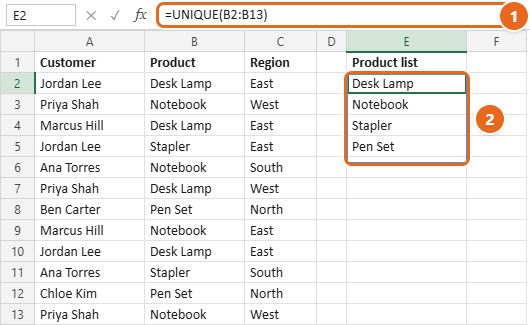
To list each customer instead, use =UNIQUE(A2:A13). It returns six names: Jordan Lee, Priya Shah, Marcus Hill, Ana Torres, Ben Carter and Chloe Kim.

Tip: Don’t include the header row in the range. If you use =UNIQUE(B1:B13), the word Product becomes the first item in your list.

Get unique rows from more than one column

When the range has more than one column, UNIQUE compares whole rows. A row is left out only when every cell in it matches an earlier row.

For example, =UNIQUE(A2:B13) returns each customer and product pair once. Jordan Lee bought a Desk Lamp twice (rows 2 and 10), and Priya Shah bought a Notebook twice (rows 3 and 13), so those two repeats are dropped. The result is 10 rows and 2 columns. Jordan Lee still appears twice in the result, once with Desk Lamp and once with Stapler, because those pairs are different.

The columns must sit next to each other in the range. To skip a column in the middle, see Use columns that aren’t next to each other below.

List values that appear only once

The third argument changes what UNIQUE returns. With exactly_once set to TRUE, any value that repeats is dropped completely, and you see only the values that occur a single time.

• =UNIQUE(A2:A13) returns all six customers, one time each. This is often called a distinct list.
• =UNIQUE(A2:A13,,TRUE) returns only Ben Carter and Chloe Kim, the two customers who placed a single order. One common use is finding customers who never came back, so you can follow up with them.

If nothing in the range appears exactly once, Excel has no results to show and returns a #CALC! error. In the sample data, =UNIQUE(B2:B13,,TRUE) does this, because every product was ordered at least twice. To show a message instead, wrap it in IFERROR: =IFERROR(UNIQUE(B2:B13,,TRUE),"No single orders").

Use UNIQUE on data that runs across a row

By default, UNIQUE compares rows, which suits lists that run down a column. If your values run across a row, set by_col to TRUE so UNIQUE compares columns instead.

Say B16:G16 holds team colors: Red, Blue, Red, Green, Blue, Red. The formula =UNIQUE(B16:G16,TRUE) returns Red, Blue and Green, and the results spill to the right. If you leave out TRUE, UNIQUE treats the single row as one record and returns it unchanged, repeats and all.

To show a horizontal result as a vertical list, wrap it in TRANSPOSE: =TRANSPOSE(UNIQUE(B16:G16,TRUE)).

Combine UNIQUE with other functions

UNIQUE is most useful as part of a bigger formula. All of these examples use the sample data and work in every version that has UNIQUE, unless a version is named.

Sort the results

Wrap UNIQUE in SORT to put the list in order:

• =SORT(UNIQUE(A2:A13)) returns Ana Torres, Ben Carter, Chloe Kim, Jordan Lee, Marcus Hill and Priya Shah.
• =SORT(UNIQUE(B2:B13),,-1) sorts Z to A: Stapler, Pen Set, Notebook, Desk Lamp. The -1 is SORT’s sort-order argument, and the empty spot before it skips the sort-index argument.

Leave out blank cells

If your range includes empty cells, UNIQUE returns one of them as a 0 in the list. This often happens when you point the formula at extra rows to leave room for new data, such as A2:A50. Use FILTER to drop blanks before UNIQUE sees them:

=UNIQUE(FILTER(A2:A50,A2:A50<>""))

The <>"" part means “not empty.” Add SORT around the whole thing for a clean, sorted list: =SORT(UNIQUE(FILTER(A2:A50,A2:A50<>""))).

List unique values that meet a condition

FILTER picks the rows that match, and UNIQUE removes the repeats:

• One condition: =UNIQUE(FILTER(B2:B13,C2:C13="East")) lists the products ordered in the East region: Desk Lamp, Stapler and Notebook.
• Both conditions (AND): multiply the tests. =UNIQUE(FILTER(A2:A13,(B2:B13="Desk Lamp")*(C2:C13="East"))) returns Jordan Lee and Marcus Hill.
• Either condition (OR): add the tests. =UNIQUE(FILTER(A2:A13,(C2:C13="North")+(B2:B13="Stapler"))) returns Jordan Lee, Ben Carter, Ana Torres and Chloe Kim.

If no row matches, FILTER returns a #CALC! error. Give FILTER its third argument to show something else, for example =UNIQUE(FILTER(A2:A13,C2:C13="Central","None")) shows None.

Count unique values

• =COUNTA(UNIQUE(A2:A13)) returns 6, the number of different customers. =ROWS(UNIQUE(A2:A13)) gives the same answer.
• =ROWS(UNIQUE(FILTER(A2:A13,C2:C13="East"))) returns 2, the number of different customers in the East region.
• If the range might contain blanks, filter them out first, as shown above. Otherwise the blank is counted as one more value.
• When a count could have no results, use =IFERROR(ROWS(UNIQUE(A2:A13,,TRUE)),0) so you see 0 instead of an error.

Count how many times each value appears

Put the unique list in one column and a COUNTIF next to it:

1. In E2, type =SORT(UNIQUE(A2:A13)).
2. In F2, type =COUNTIF(A2:A13,E2#). The # after E2 is the spilled range operator. It means “the whole spill range that starts in E2.”

F2 spills a count beside each name: Ana Torres 2, Ben Carter 1, Chloe Kim 1, Jordan Lee 3, Marcus Hill 2 and Priya Shah 3. Both lists grow or shrink together when the data changes. In Microsoft 365, the GROUPBY function can build this kind of summary in a single formula. Other counting methods are in counting the number of occurrences in Excel.

List values that appear more than once

To see only the repeated entries, each shown once, combine FILTER and COUNTIF:

=UNIQUE(FILTER(A2:A13,COUNTIF(A2:A13,A2:A13)>1))

This returns Jordan Lee, Priya Shah, Marcus Hill and Ana Torres. Change >1 to >2 to list only customers with three or more orders.

Join two columns into one list

Use the & operator to join columns before UNIQUE compares them. =UNIQUE(A2:A13&" ("&C2:C13&")") returns one text entry per customer and region pair, such as Jordan Lee (East) and Ana Torres (South). The result is a single column of text, which is handy for labels or a drop-down list.

Use columns that aren’t next to each other

To get unique Customer and Region pairs while skipping the Product column in between:

• Microsoft 365 and Excel 2024: =UNIQUE(CHOOSECOLS(A2:C13,1,3)). CHOOSECOLS keeps the first and third columns of the range.
• Excel 2021: =UNIQUE(FILTER(A2:C13,{1,0,1})). The {1,0,1} tells FILTER to keep the first and third columns and drop the second.

Both return six rows, one for each customer with their region.

Combine two lists

In Microsoft 365 and Excel 2024, VSTACK stacks ranges on top of each other so UNIQUE can treat them as one list. If you have a second list of customers in H2:H8, =SORT(UNIQUE(VSTACK(A2:A13,H2:H8))) returns every customer from both lists once, in A to Z order. Excel 2021 doesn’t have VSTACK, so copy one list under the other first.

Keep the list up to date as data grows

UNIQUE updates when cells inside its range change, but it doesn’t stretch to include new rows added below the range. If you add a 13th order in row 14, =UNIQUE(A2:A13) won’t see it. There are two good fixes:

• Use an Excel table (recommended). Click inside your data, press Ctrl+T, and select OK. If the table is named Orders, use =UNIQUE(Orders[Customer]). With structured references like this, the result resizes automatically as you add or remove rows. To name a table, click in it and type a name in Table Name on the Table Design tab. More on tables is in creating a table in Excel.
• Use a larger range and filter out blanks. For example, =UNIQUE(FILTER(A2:A500,A2:A500<>"")) covers up to 499 rows of data and ignores the empty ones. In Microsoft 365, TRIMRANGE is another way to trim empty rows off a large range.

Important: Put the UNIQUE formula outside the table, in a normal part of the sheet. Spilled formulas aren’t supported inside Excel tables and show #SPILL! there.

Build a drop-down list from UNIQUE

A UNIQUE list makes a good source for a drop-down, because it never shows the same choice twice and it updates when the data changes.

1. Create the list. In E2, enter =SORT(UNIQUE(B2:B13)). It spills Desk Lamp, Notebook, Pen Set and Stapler into E2:E5.
2. Select the cell for the drop-down. Click the cell where people should pick a product, such as H2.
3. Open Data Validation. Select Data > Data Validation in the Data Tools group. The Data Validation dialog box opens on the Settings tab.
4. Choose List. In the Allow box, choose List. Leave In-cell dropdown checked.
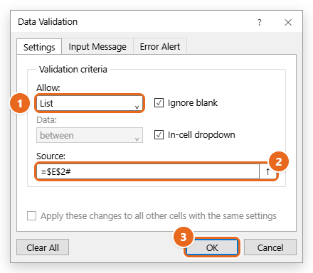
5. Enter the spill reference. In Source, type =$E$2#, including the # sign, then select OK.
   

   

6. Test it. Click H2 and select the arrow. You see the four products. Add a new product to column B, inside the range or table that UNIQUE reads, and it appears in the drop-down without changing the validation settings.

Creating a drop-down list in Excel covers more ways to set up and edit drop-downs.

Turn the results into fixed values

A UNIQUE list keeps changing with the source. If you need a snapshot that stays put, for example to send to someone or to sort and edit by hand:

1. Select the whole spill range, such as E2:E5, and press Ctrl+C (Command+C on a Mac).
2. Click where you want the fixed list. It can be the same place.
3. Select Home > the arrow under Paste > Paste Values (the clipboard icon with 123). The values stay and the formula is gone.

To remove a UNIQUE list entirely, select the first cell of the spill range, E2 in the example, and press Delete. The whole spill range clears. Deleting E3 or another cell further down the list doesn’t work, because only the first cell holds the formula.

Troubleshooting

#SPILL! error

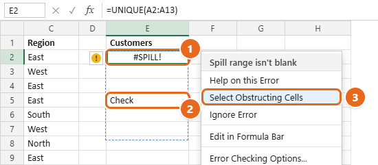
Excel can’t place the results because something is in the way. The most common cause is a value, a space or a formula in one of the cells the list needs. Select the cell with the error to see a dashed border around the area Excel wants to fill.

1. Select the cell that shows #SPILL!.
2. Select the yellow warning icon that appears next to it.
3. Choose Select Obstructing Cells. Excel jumps to the cell that’s in the way.
   

   

4. Delete or move that cell’s contents. The list appears as soon as the space is clear.

The same error also appears when the formula is inside an Excel table, when the results would land on merged cells, and when the results would run past the edge of the worksheet, as the #SPILL! error article explains. Move the formula out of the table, unmerge the cells, or use a smaller range instead of a whole column.

#NAME? error

Your version of Excel doesn’t have UNIQUE, or the function name is misspelled. UNIQUE needs Microsoft 365, Excel 2024, Excel 2021, Excel for the web or the mobile apps. In Excel 2019 or earlier, use Data > Remove Duplicates or Data > Advanced with Unique records only instead. Both are covered in removing duplicates in Excel.

#CALC! error

There are no results to show. This happens with exactly_once set to TRUE when every value repeats, or with FILTER when no row matches. Use IFERROR, or FILTER’s third argument, to show a message instead.

A 0 appears in the list

The range includes at least one empty cell. Filter out blanks with =UNIQUE(FILTER(A2:A50,A2:A50<>"")).

Values that look the same are listed twice

• Extra spaces. Ana Torres with a space at the end is different from Ana Torres without one. Use =UNIQUE(TRIM(A2:A13)) to remove extra spaces as you go.
• Numbers stored as text. The text 10 and the number 10 count as two different values. Cells with a small green triangle in the corner are often numbers stored as text. Select them, select the warning icon, and choose Convert to Number.
• Different spellings. UNIQUE only matches identical text, apart from capital letters. Jordan Lee and Jordon Lee are two values.

#REF! after closing another workbook

Dynamic array formulas linked to another workbook only work while both files are open. If you close the source workbook, the formula shows #REF! when it recalculates. Open the source file again, or copy the data into the same workbook.

New rows aren’t included

The range in the formula ends above the new data. Convert the data to a table or use a larger range, as described in Keep the list up to date as data grows.

FAQ

Which versions of Excel have the UNIQUE function?

UNIQUE is available in Excel for Microsoft 365 on Windows and Mac, Excel 2024, Excel 2021 (Windows and Mac), Excel for the web, and Excel for iPhone, iPad and Android. Excel 2019, 2016 and earlier don’t have it.

What’s the difference between unique and distinct values?

In everyday use, both mean “each value once,” which is what =UNIQUE(range) returns. Strictly speaking, in database terms “unique” means values that occur exactly one time. That’s what you get with =UNIQUE(range,,TRUE).

Is UNIQUE case-sensitive?

No. UNIQUE treats SALES, Sales and sales as the same value and keeps whichever version appears first. There’s no setting to change this. If capital letters matter, for example in product codes, Power Query’s Remove Duplicates command is case-sensitive.

Does UNIQUE change or delete my original data?

No. It only reads the range and writes its results somewhere else. To delete duplicate rows from the data itself, use the Remove Duplicates button.

Can I use UNIQUE inside an Excel table?

Not as a spilled list. A UNIQUE formula entered in a table cell shows #SPILL!. You can point UNIQUE at a table column, such as =UNIQUE(Orders[Product]), as long as the formula itself sits outside the table.

How do I count unique values in Excel?

Use =COUNTA(UNIQUE(range)) or =ROWS(UNIQUE(range)). To count only values that appear once, use =ROWS(UNIQUE(range,,TRUE)) inside IFERROR in case there are none.

Can I reference the UNIQUE results in another formula?

Yes. Add # after the first cell of the spill range, such as =COUNTA(E2#) or =COUNTIF(A2:A13,E2#). The reference grows and shrinks with the list. The article on the spilled range operator has more examples.

Next step

Try =SORT(UNIQUE(range)) on a column in one of your own sheets, with plenty of empty space below the formula. Once that works, format your data as a table so the list keeps up as you add rows, and use the spill reference to feed a drop-down list or a count.